Tutorial 2 - Simple 2D Calculation
1. Task - Exterior Wall with Intersecting Interior Wall
This tutorial shows how 2D construction details can be simulated with DELPHIN 6.1.8. A simple thermal bridge is modeled and calculated for this purpose.
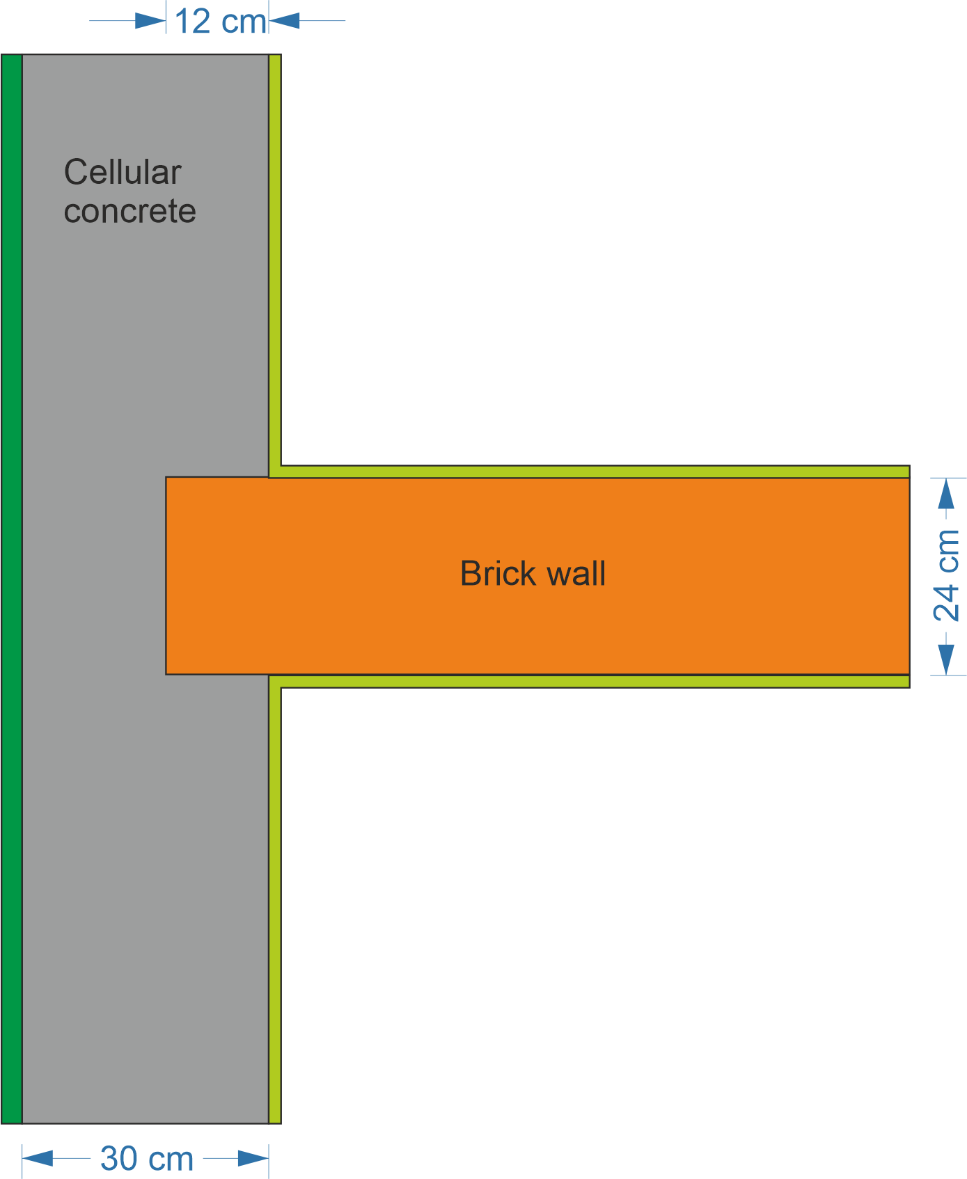
The construction detail shown below represents an interior wall intersecting an exterior wall and is to be calculated in DELPHIN. The exterior wall consists of aerated concrete, while the interior wall is made of brick masonry.
1.1. Simplification of the Construction Detail
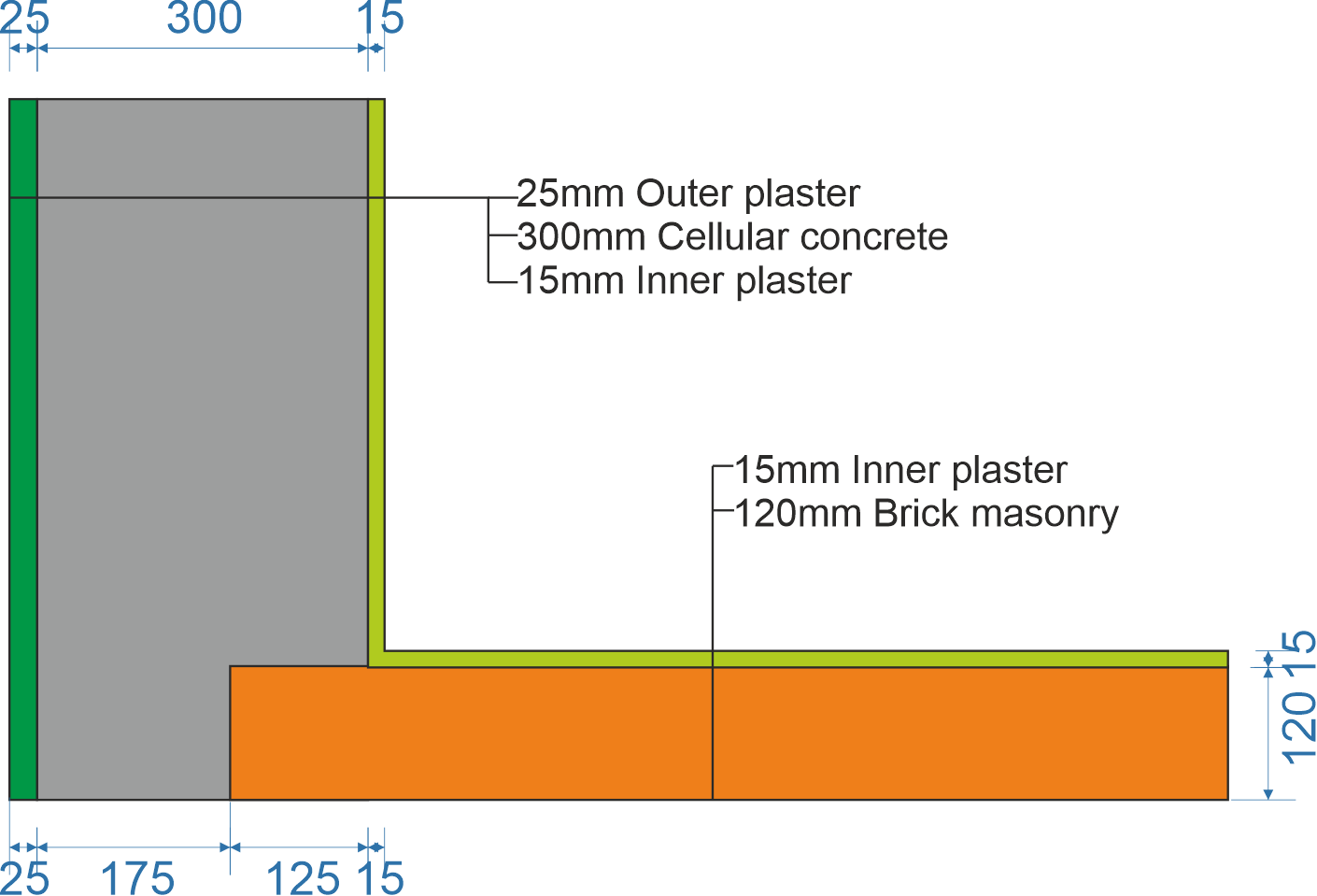
Before entering a construction in DELPHIN, it should be examined whether the model can be simplified. One option in this example is to make use of axes of symmetry and to place the model boundary along such an axis. This reduces the number of discretized elements and therefore the simulation time.
1.2. Generating the Construction Grid
In DELPHIN, constructions are developed on a rectangular grid. First, the construction lines are defined. Materials are then assigned to the individual cells, or the cells remain empty, for example in the case of an opening. The following grid represents the construction:
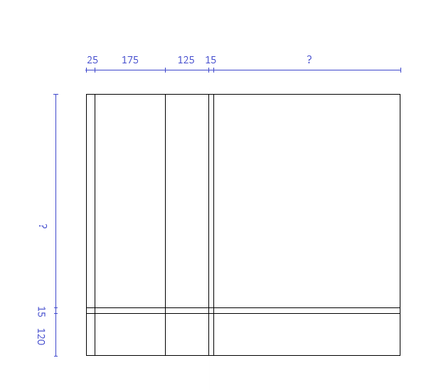
Values are still required for the length/width marked “? cm”. The modeled lengths of the exterior and interior walls must be selected large enough that the influence of the thermal bridge on the temperature field is no longer relevant. According to EN ISO 10211, a length of one meter or three times the wall thickness should be used, whichever is greater. Here, 100 cm is selected for both the exterior wall and the interior wall. If the simulation results show that the ends of the one-dimensional wall sections are still influenced by the thermal bridge, the detail must be enlarged.
2. Input in DELPHIN
2.1. General Input
The modeling procedure initially follows Tutorial 1. When creating the project, leave the project information blank. Select a hygrothermal simulation (standard), set the calculation period to 2 years, and select Potsdam as the climate location.
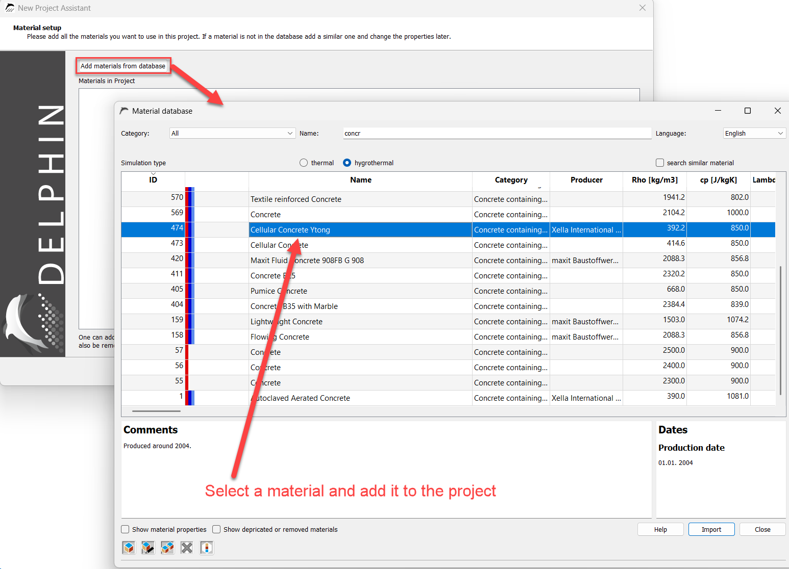
For the materials, any aerated concrete (e.g. 474) and a standard brick (e.g. 512) can be selected. A lime interior plaster (e.g. 681) is used for the interior plaster and a lime-cement plaster (e.g. 145) for the exterior plaster.
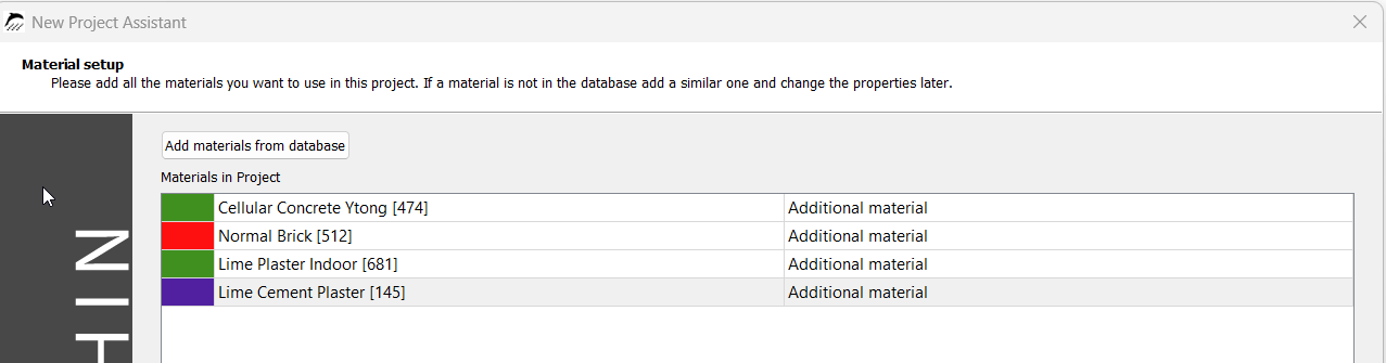
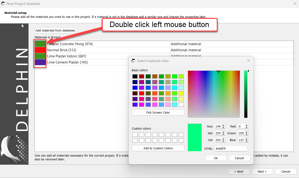
Starting with DELPHIN version 6.1.8, material colors can already be selected in this dialog. Double-click the color field of the respective material with the left mouse button; a window opens in which the desired color can be selected.
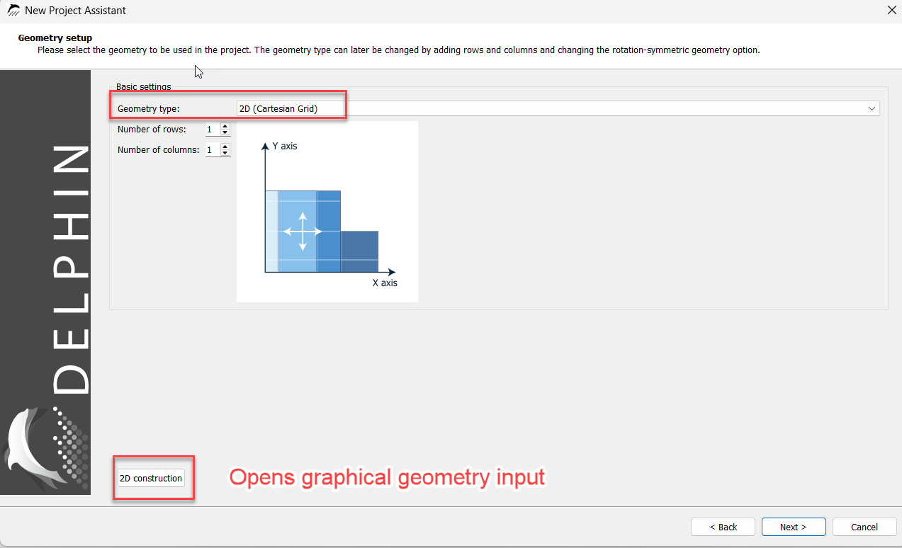
Then select '2D (Cartesian coordinate system)' in the geometry specification window.
2.2. Graphical Geometry Input
To simplify input, DELPHIN 6.1.8 provides a graphical input function that can be opened by clicking the “2D Construction” button at the lower left of the window. The number of rows and columns can be ignored at this point, as these values are updated automatically after the 2D geometry has been created using the graphical interface.
The construction dialog provides various functions, which are briefly explained below:

1: Add horizontal guide lines
2: Add vertical guide lines
3: Overview of all existing guide lines, changing positions, and deleting
4: Create a guide line at a specified distance from an existing guide line
5: Overview of all assigned materials (position, height, width, remove material)
6: Move the selected material one layer forward
7: Move the selected material one layer backward
8: Display a grid in the background
9: Zoom in
10: Zoom out
11: Show the complete view
12: Zoom into a selected area (click icon 12 -→ mark an area in the drawing window while holding the left mouse button -→ release the mouse button)
13: Show/hide guide lines
14: Undo
15: Redo
The previously selected materials and a field named “VOID” are shown on the right-hand side. VOID can be used to model cavities in the construction, for example where pipes or similar elements are required.
2.2.1. Coordinate System and Guide Lines
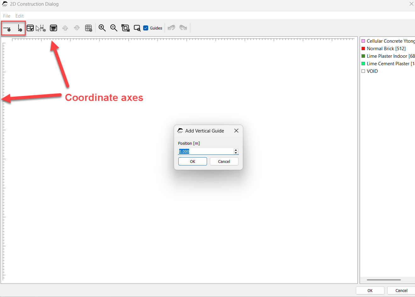
A coordinate system is also displayed on the screen, with its origin at the lower left of the window.
This provides orientation when creating the sketch.
Guide lines can be created in two ways. Click an axis with the left mouse button, for example the horizontal axis, and drag the mouse downward while holding the button. Release the mouse button to place the guide line at the desired position.
Guide lines can also be created by clicking the first icon from the left (horizontal guide line) or the second icon from the left (vertical guide line). A window opens in which the guide-line position is entered. This value specifies the distance from the corresponding parallel coordinate axis.
Clicking a guide line with the left mouse button turns it red, indicating that it is selected. Clicking the guide line again opens a window showing its position as the distance from the axis. The guide-line position can be entered manually in the yellow field.
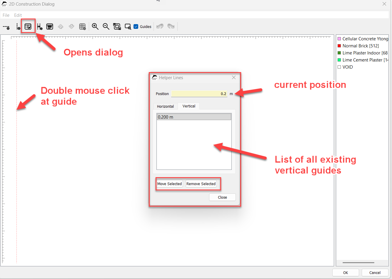
The positions of other guide lines are also visible in this window. The window can also be opened using the third button from the left in the toolbar.
Guide lines can also be deleted in this window. Select the relevant guide line with a left click and then delete it using the “Remove selected object” button.
2.2.2. Additional Settings
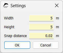
Clicking “File” at the upper left of the window allows guide lines to be saved and previously saved guide lines to be loaded. Under “Edit”, settings for the graphical construction can be opened, such as the width and height of the drawing area and the snap distance.
Zooming in the construction area is performed using the mouse wheel.
2.3. Creating the Example Construction
2.3.1. Creating Guide Lines
The construction is now created as follows:
First, guide lines are created so that the construction can be represented according to the dimensions shown above.
The first guide line is created by clicking the second icon from the left in the toolbar. The distance from the coordinate system can be selected freely and is set to 0.1 m in this example. This guide line marks the left side of the exterior wall.
A second guide line is placed at a distance of 0.125 m from the coordinate system. This layer represents the exterior plaster with a thickness of 2.5 cm. A third guide line is then created at a distance of 0.275 m from the second guide line.
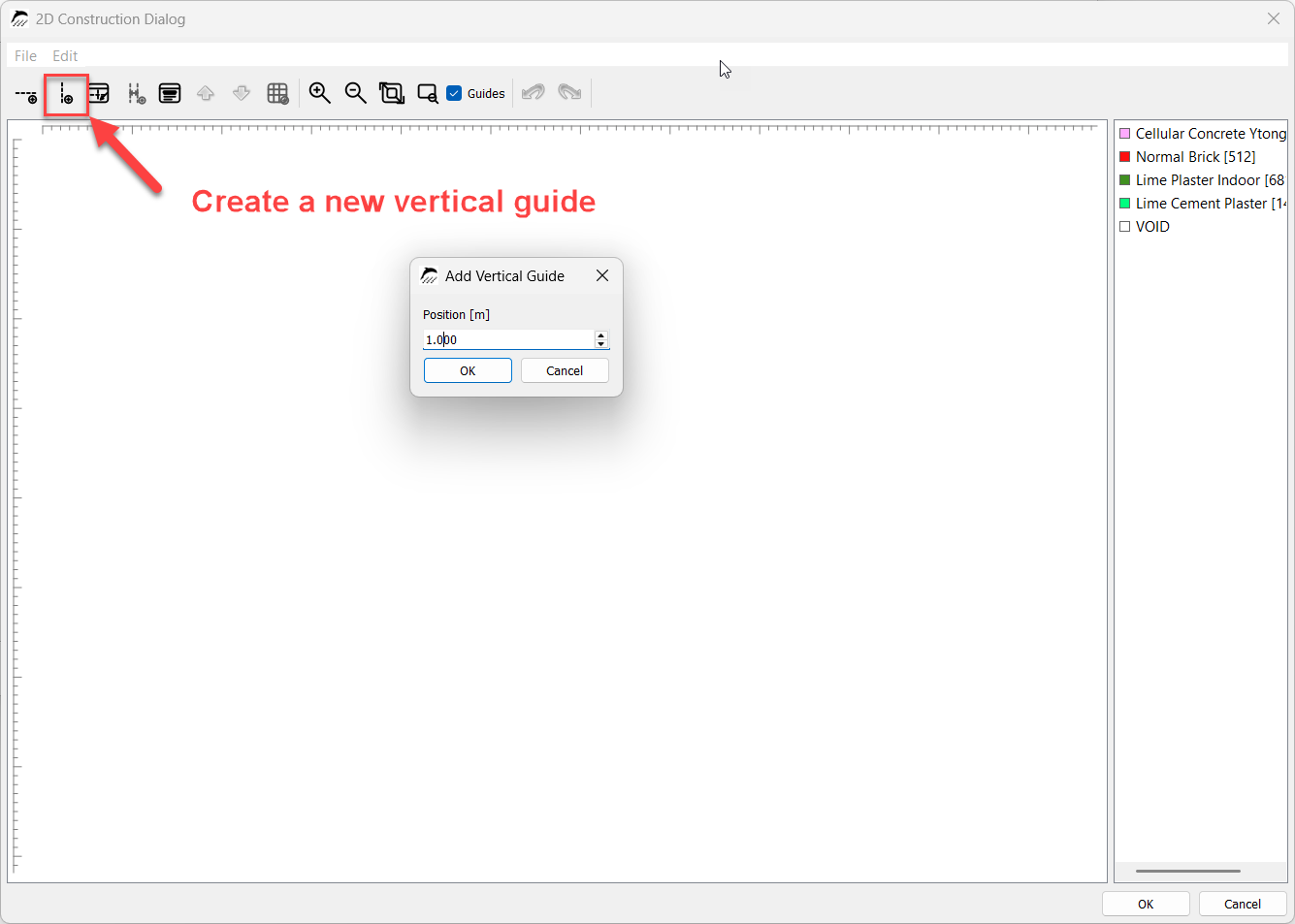
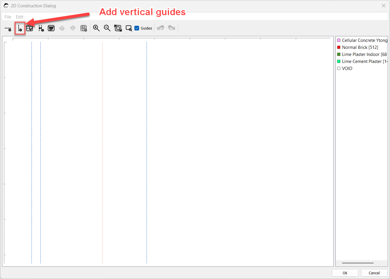
The fourth guide line marks the point to which the brick masonry extends into the aerated concrete. A guide line is therefore placed at a distance of 0.425 m from the vertical coordinate axis. Finally, a fifth guide line is created to mark the inner face of the interior plaster. It is located 0.44 m from the coordinate axis.
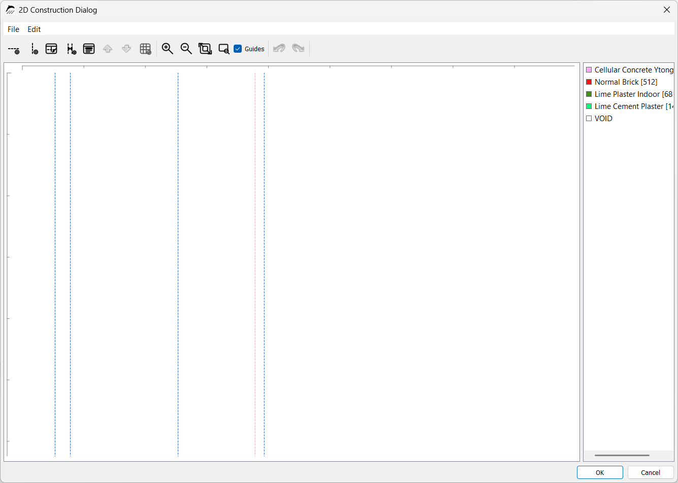
Placing guide lines at the desired distance
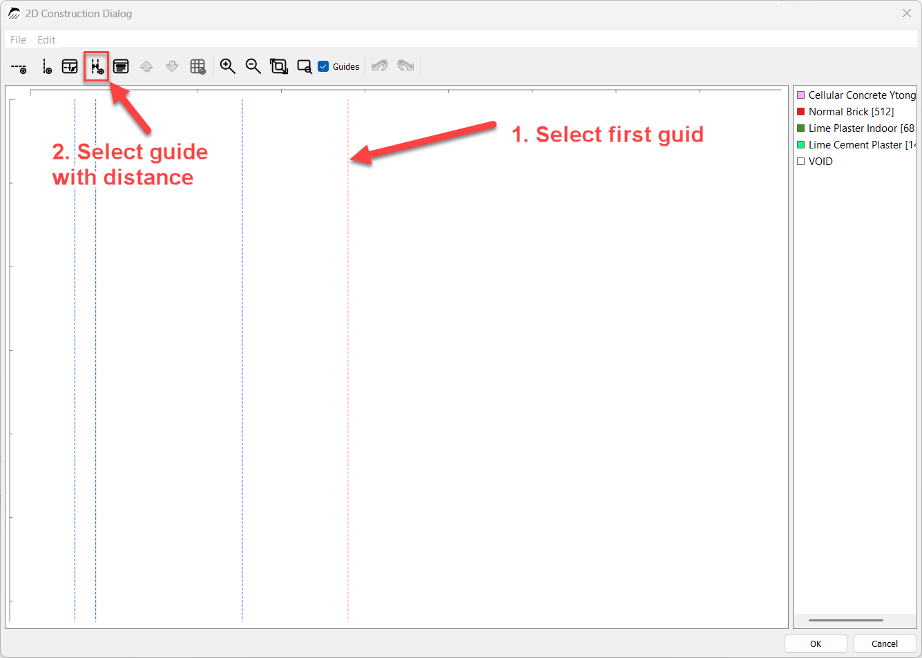
Another way to create the second and third guide lines is to add them at a specified distance from the first guide line. This can be done using the fourth button in the toolbar. In this case, the distance of the first guide line from the coordinate axis does not need to be considered. For this example, a distance of 0.025 m would therefore be selected for the second guide line and 0.175 m for the third guide line. To place a guide line at a specified distance, first select the relevant guide line and then click the fourth button in the toolbar. Enter the desired distance, confirm with “OK”, and click once on the side of the guide line where the new guide line is to be created. The new guide line now appears at the specified distance.
2.3.2. Adding Materials
The materials can now be added. Add the “Aerated concrete” material for the exterior wall by clicking it with the left mouse button and dragging it into the construction area while holding the mouse button. When the mouse button is released, a window opens in which the material dimensions can be entered. Here, a width of 0.3 m and a height of 1.12 m are selected.
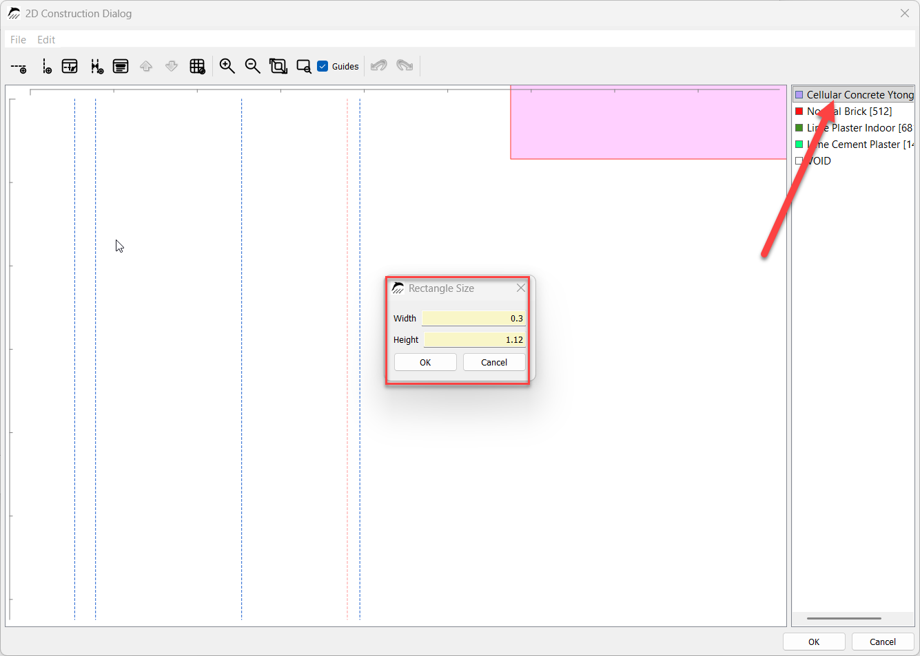
The material must now be positioned accordingly. There are two options:
Clicking the material area allows the material to be moved to the left guide line. A snap function positions the material on the guide line. More precise control is possible by clicking the left edge of the rectangle. This is particularly useful when different materials are to be placed next to each other without overlap. The material can then be moved.
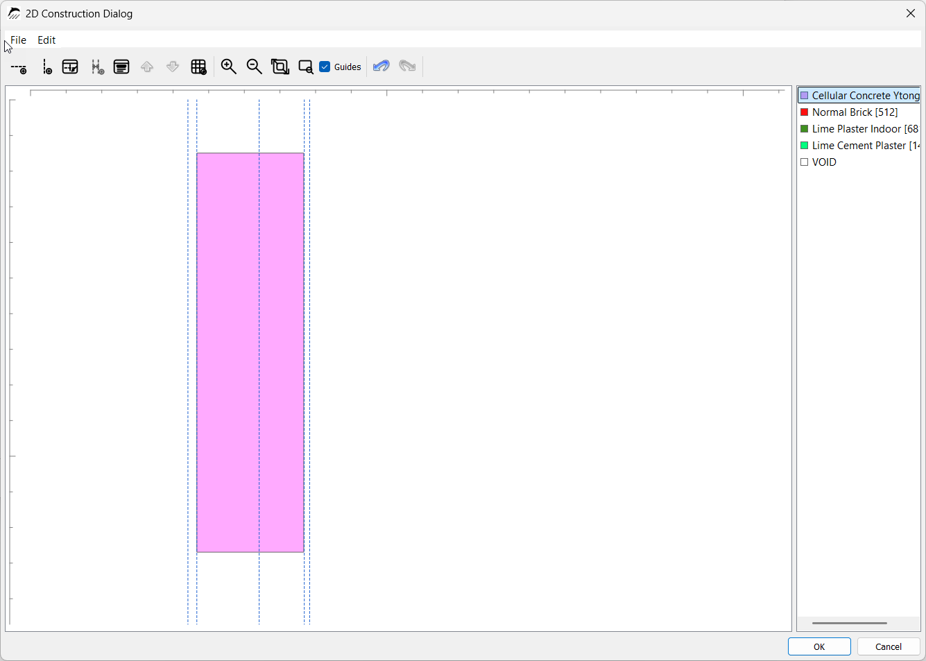
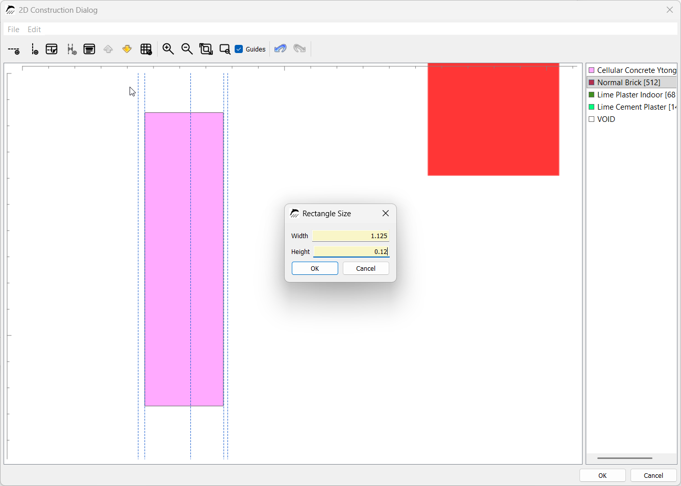
The interior wall is then added by dragging the corresponding “Standard brick” material into the drawing area. The brick wall has a height of 0.12 m and a length of 1.125 m. The length consists of the 100 cm brick-wall length within the room plus the 12.5 cm embedment depth into the aerated concrete wall, resulting in a total length of 1.125 m. Click the left outer edge and move the material to the second guide line.
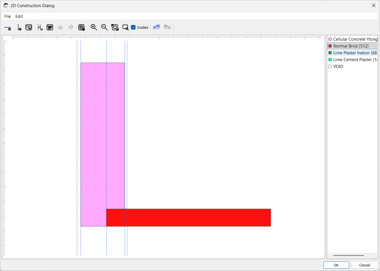
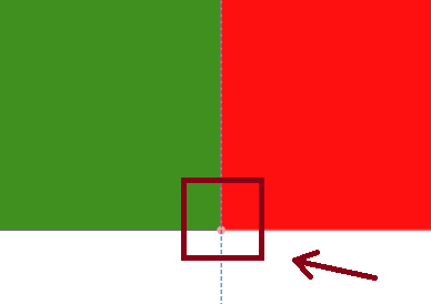
For more precise positioning, click the lower-left corner and move the material flush to the intersection between the exterior wall and the guide line.
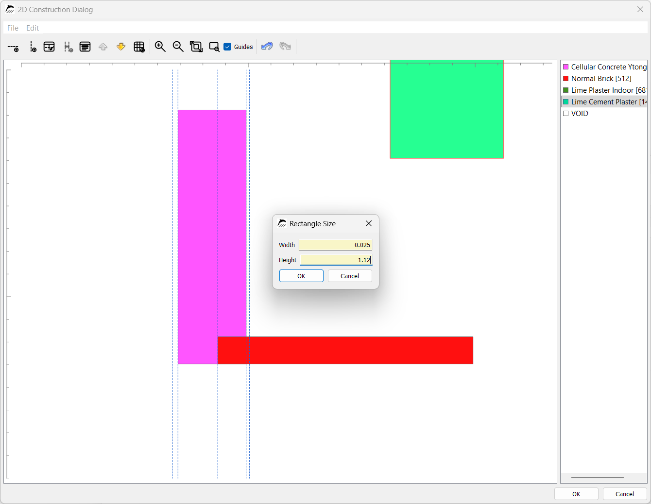
The interior and exterior plaster are then added. Drag the “Lime-cement plaster” material into the drawing area. It is assigned a width of 0.025 m and, like the aerated concrete, a height of 1.12 m.
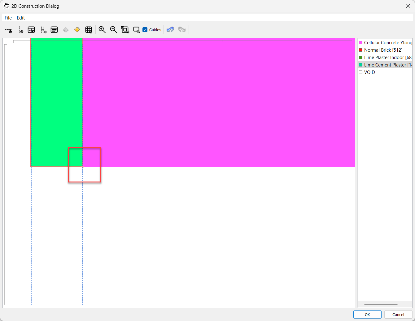
The interior plaster must now be assigned to both interior edges. On the inner side of the aerated concrete, it has a thickness (width) of 0.015 m and a height of 1.00 m. It is then positioned accordingly.
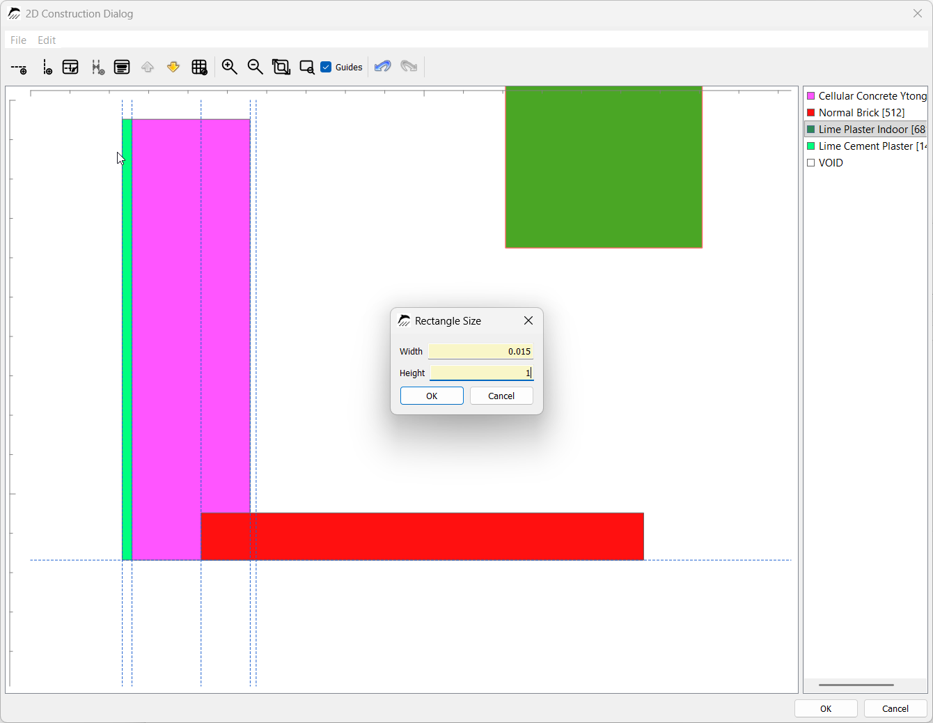
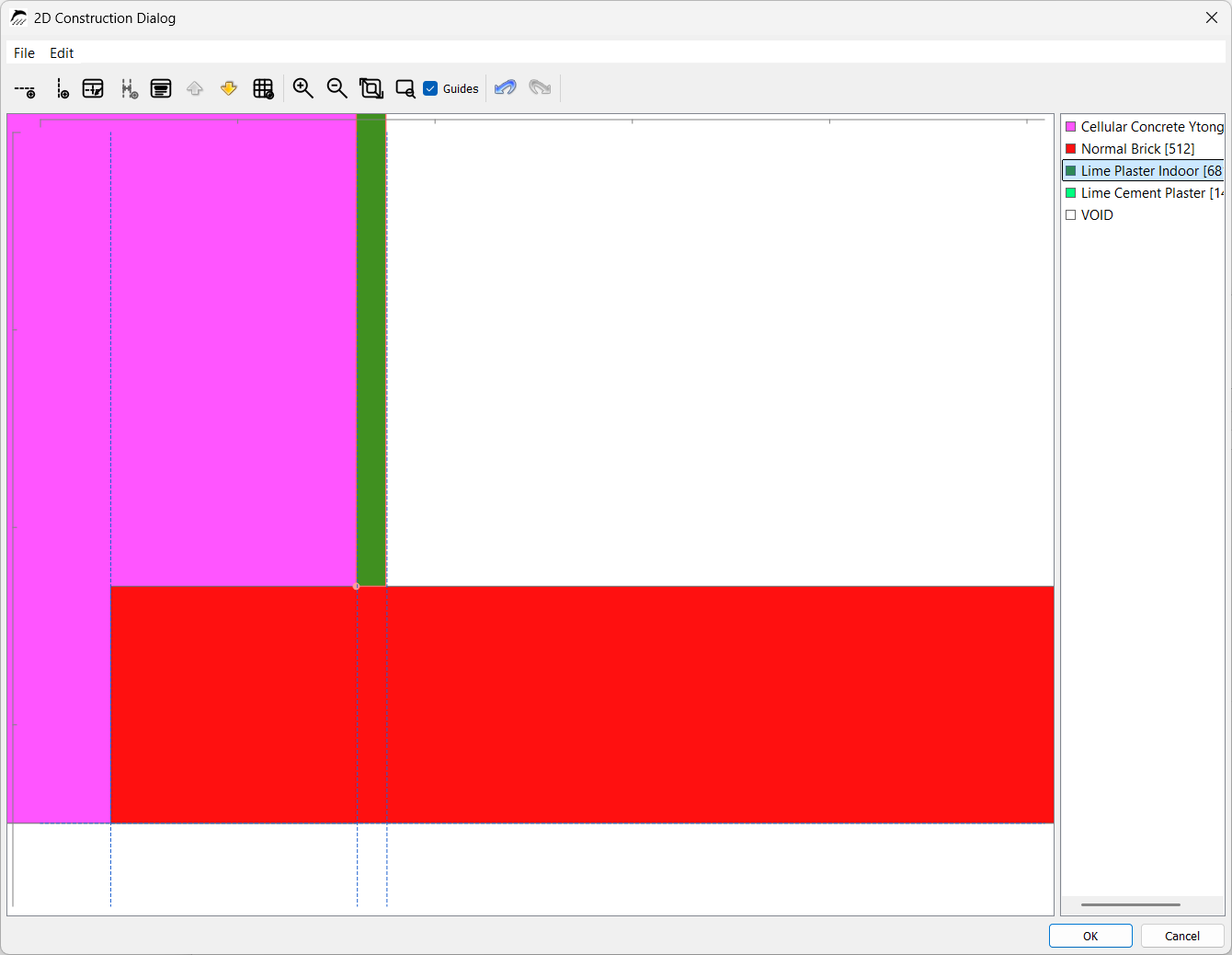
Interior plaster with a thickness (height) of 0.015 m and a width of 1.00 m is also assigned to the brick masonry.
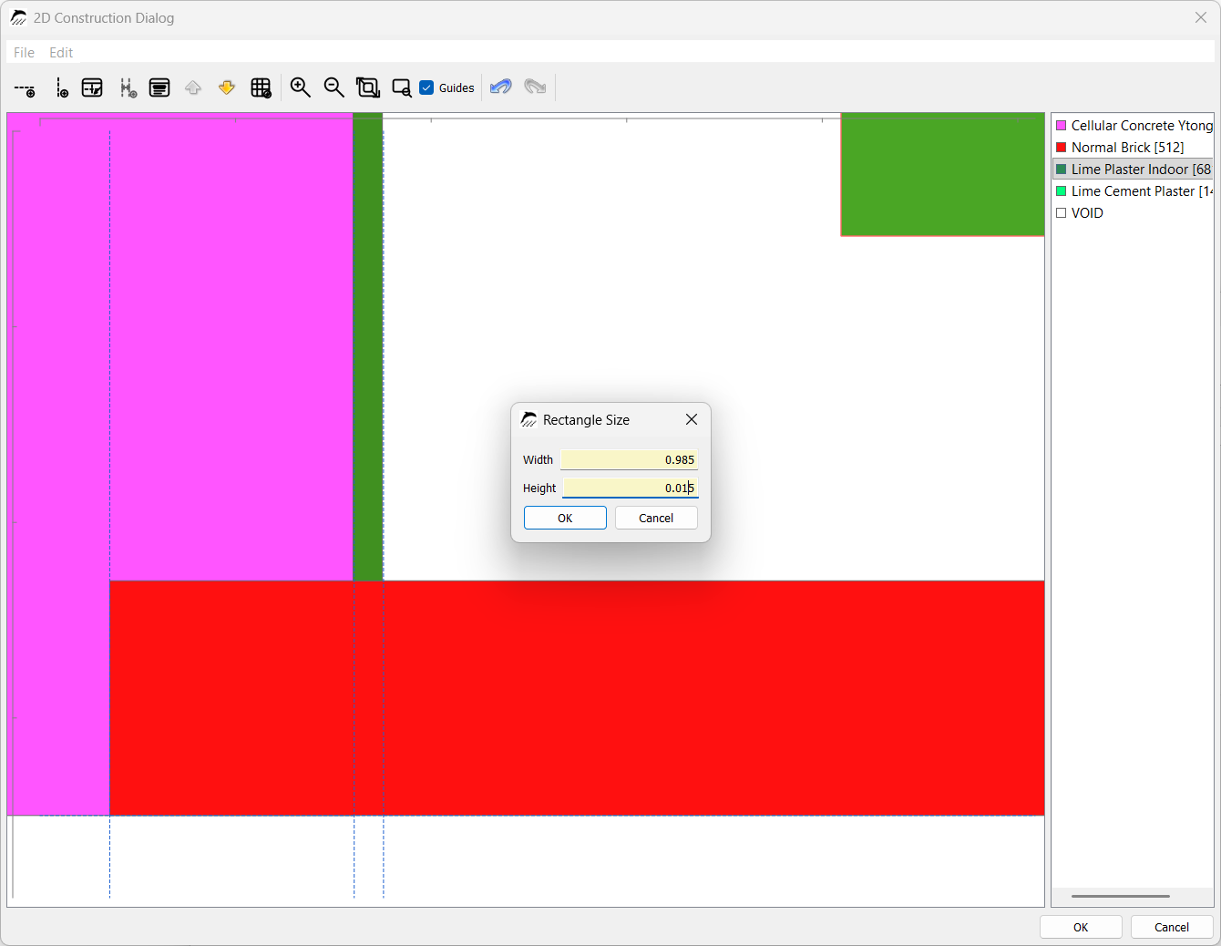
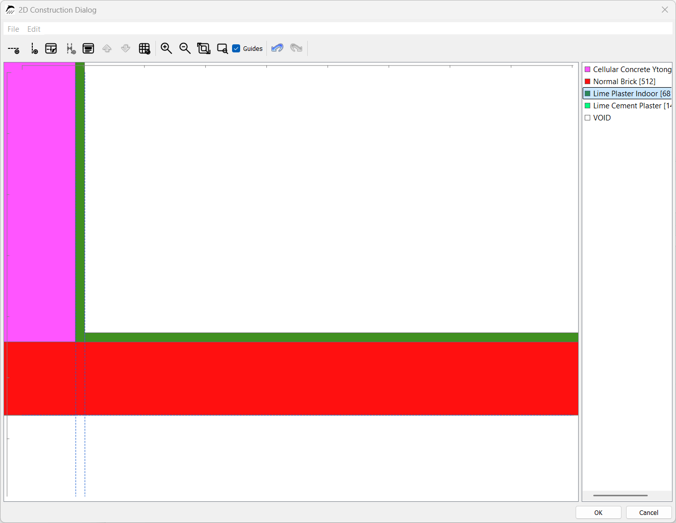
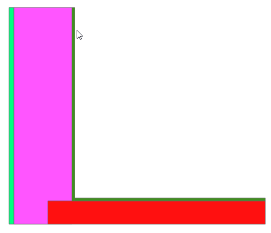
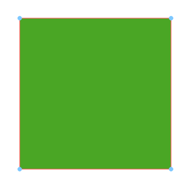
The elements can be resized afterwards. Hold [Shift] and click the desired material area to activate a mode for resizing the area. The materials can then be enlarged or reduced using the corner points.
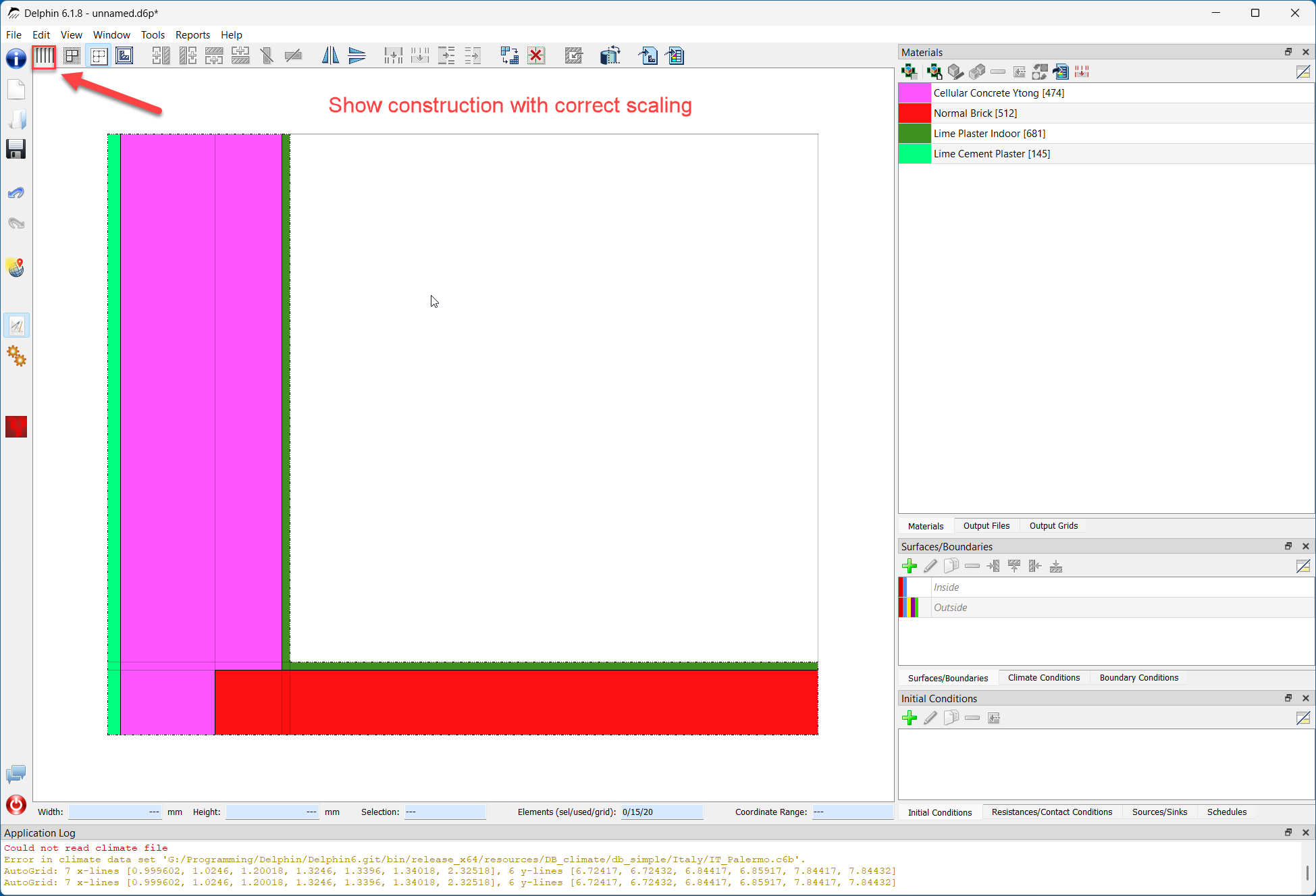
The construction is now complete. Click “OK” to close the window. A small preview of the created construction is now visible at the lower right of the project creation wizard.
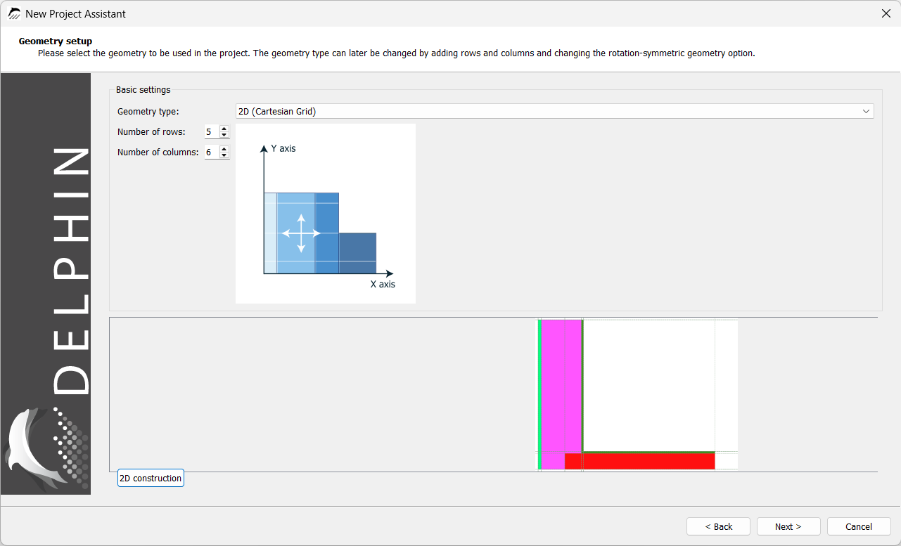
As in the previous DELPHIN version, it is also possible to first create a grid from a specified number of columns and rows and then assign the materials as usual after completing the wizard. This is described in the appendix. Layer thicknesses and heights can also be changed later at any time, and layers can be added or deleted.
2.3.3. Surfaces and Predefined Outputs
Click “Next” to configure the boundary conditions in the next step. For 2D constructions, these are created by the wizard but must subsequently be assigned to the corresponding locations in the program.
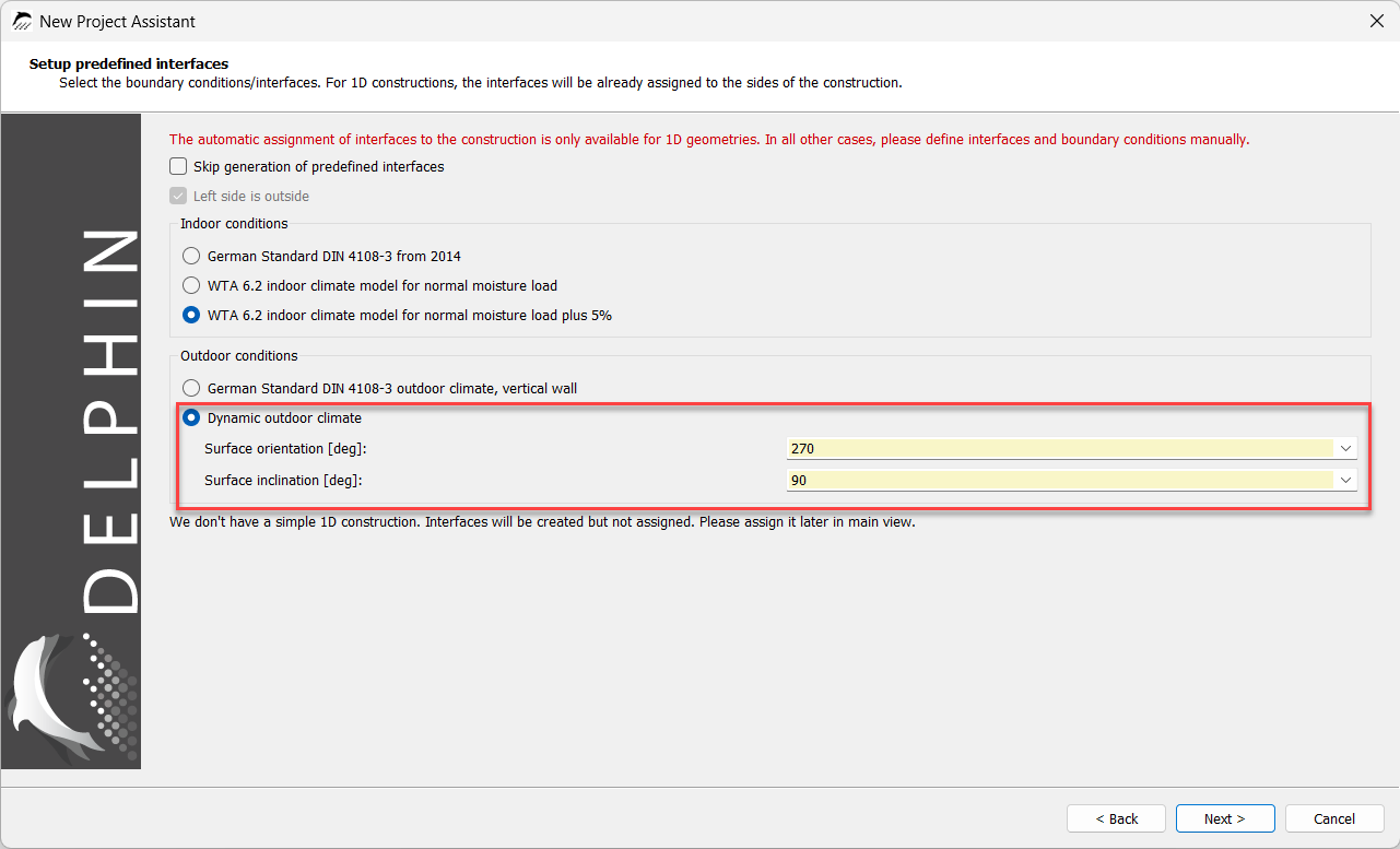
The orientation and inclination of the construction surface are also specified here. Since this is a wall, an inclination of 90° is selected. The project creation wizard creates the exterior boundary condition for only one orientation. Therefore, for a project with two exterior walls and different orientations (e.g. an exterior wall corner), a second exterior boundary condition must be created after completing the project wizard. This is described later in the tutorial in Assigning Boundary Conditions. Here, select an orientation of 270° for the west wall and click “Next”.
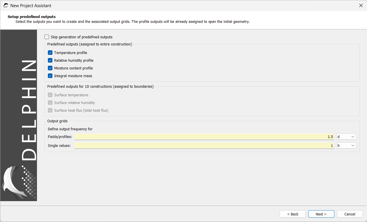
Compared with older DELPHIN versions, predefined outputs can now be generated. They can be selected in this window and refer to the entire construction.
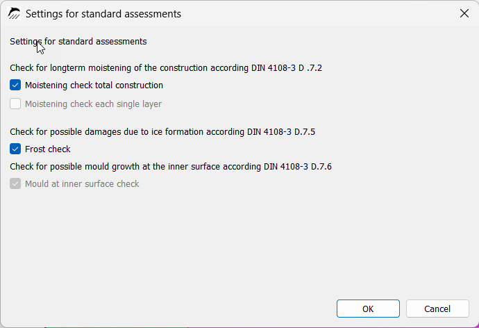
Additional settings for standard assessments can be made in the next window. Moisture accumulation and frost-damage checks can be added for the complete construction. The mold-growth assessment cannot yet be enabled at this point because the interior and exterior surfaces of the model have not yet been defined.
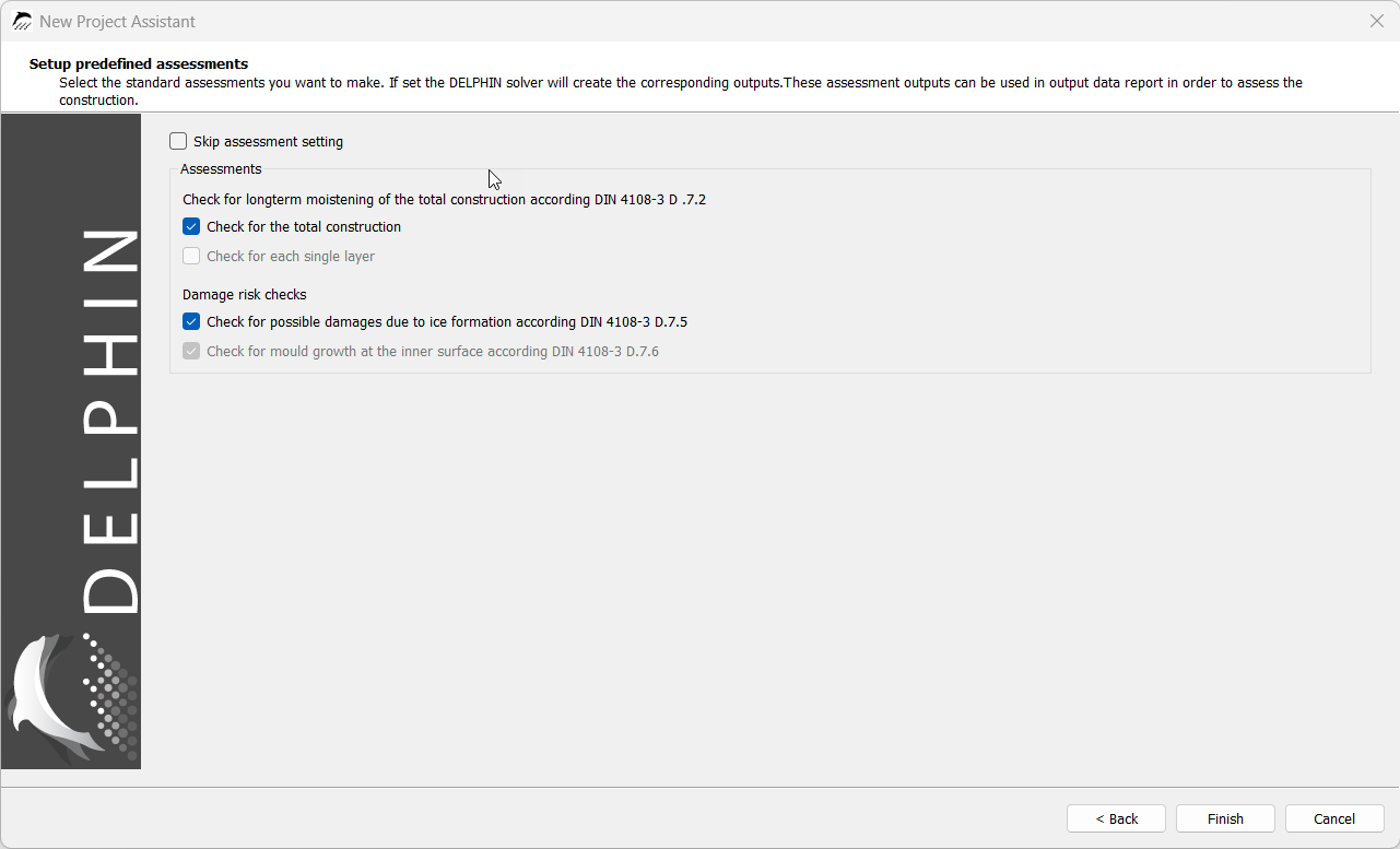
The wizard can then be closed.
The construction is now visible. If errors occurred while creating the construction using the drawing function, they can be corrected here. This procedure is unchanged from the previous DELPHIN version and is described in the appendix.
2.4. Assigning Boundary Conditions
In this section, surface conditions are assigned to selected boundaries of the modeled construction. The following sketch illustrates the boundary conditions and the associated climatic conditions for temperature and relative humidity at the surfaces.
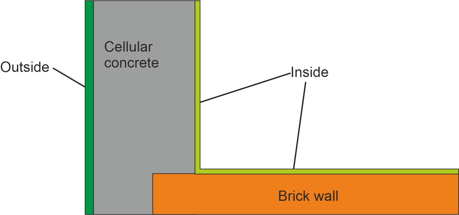
Boundary conditions are not required at axes of symmetry and at boundaries of the computational domain where one-dimensional conditions are expected. A boundary without a climate boundary condition is treated as completely impermeable and adiabatic. Heat and vapor boundary conditions must be created and assigned to the other two boundaries.
An interior and an exterior boundary condition have already been created. Double-click the interior boundary condition to open it and select the corresponding indoor climate model.
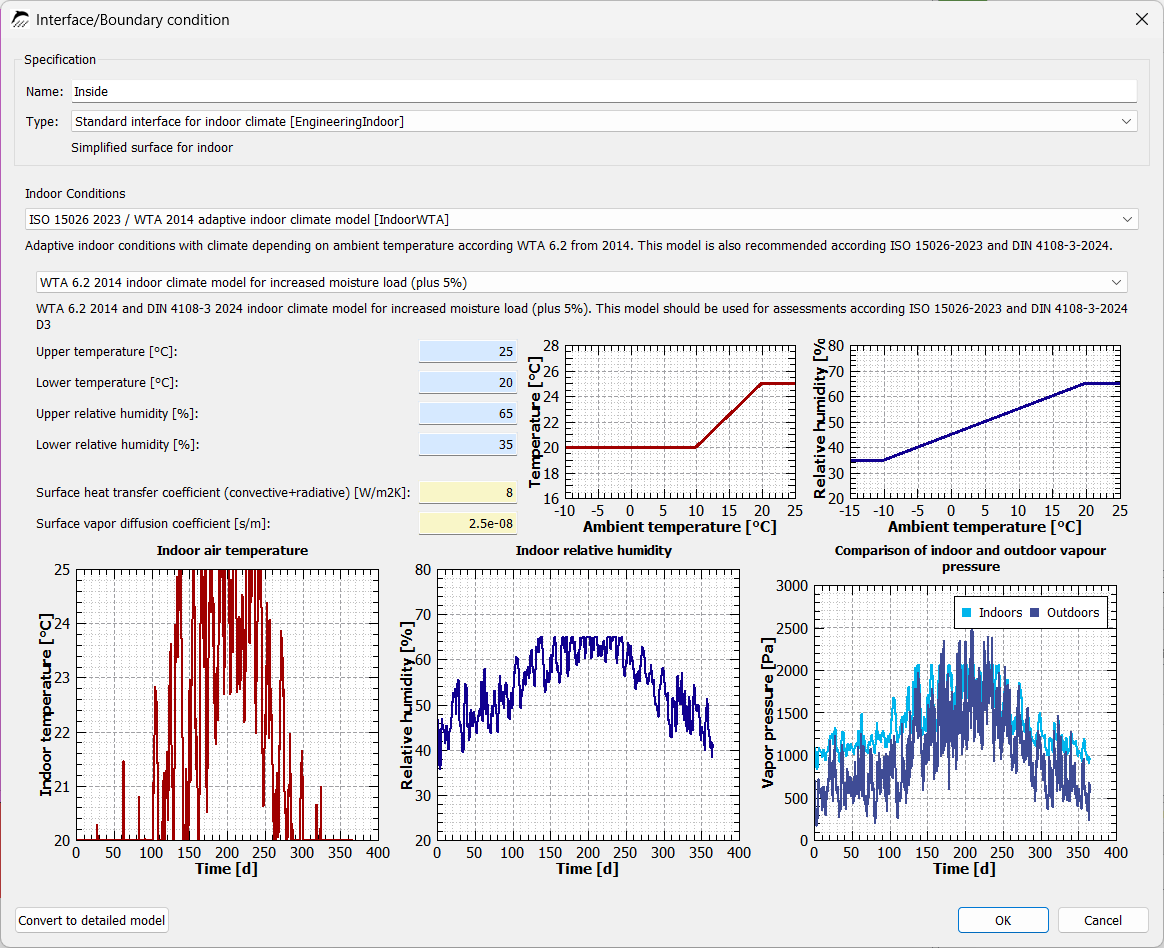
In this example, the indoor climate according to WTA 6.2:2025 is selected. The moisture load can be set to “increased moisture load” to represent the most critical case.
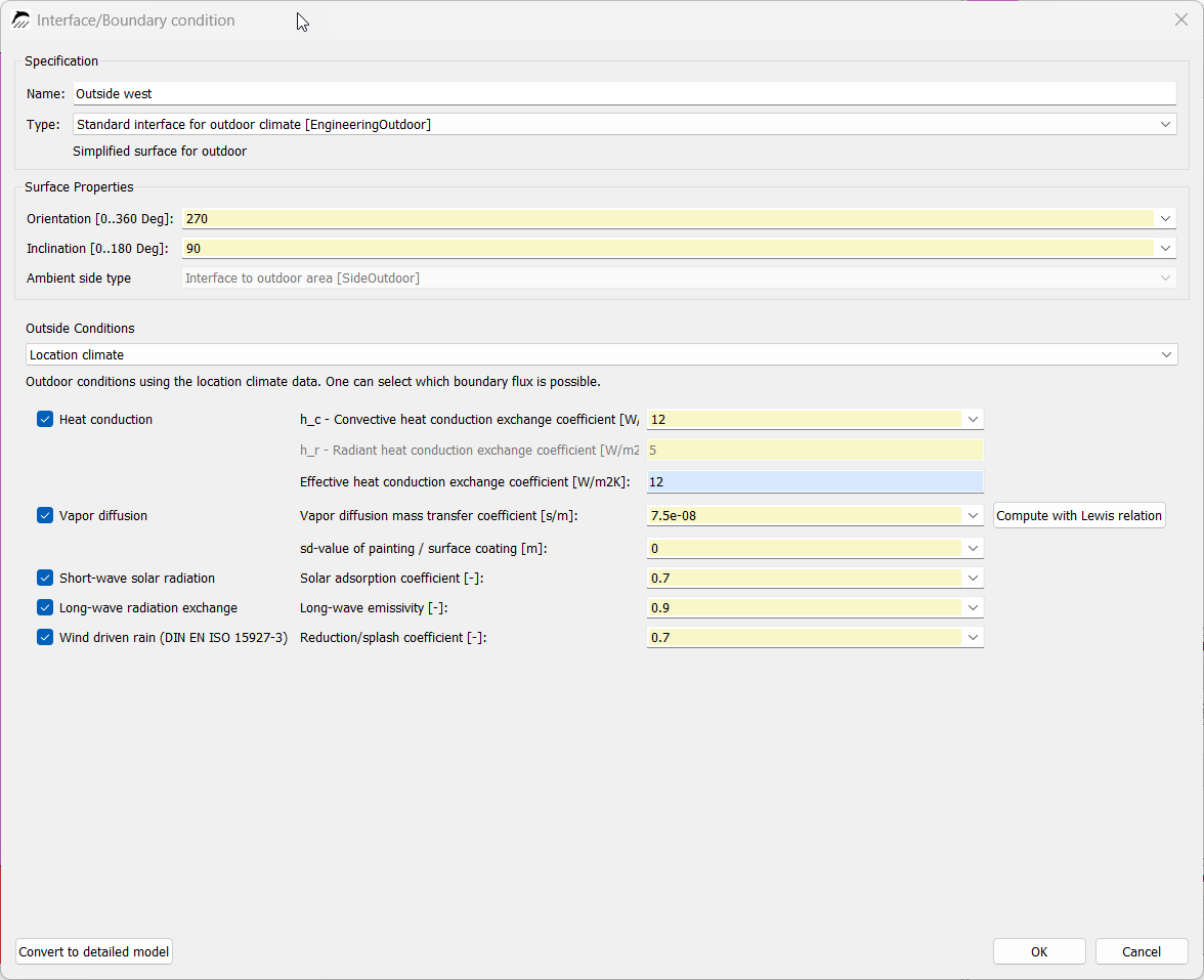
The outdoor climate can likewise be opened by double-clicking it. Driving rain and radiation are neglected in this example and can therefore be disabled by clearing the blue check boxes.
Creating a second exterior boundary condition:
For some constructions, such as the calculation of an exterior wall corner, it may be necessary to create multiple exterior boundary conditions.
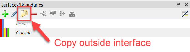
For this purpose, two exterior boundary conditions with different orientations must be created, for example facing north and west. To assign the exterior boundary conditions in this case, a second boundary condition for the north wall must first be created by copying the existing exterior boundary condition. The boundary conditions should be named unambiguously, for example by adding “North” and “West” to their names. Set the orientation to 0° to simulate climatic conditions on the north side. The window can then be closed and the boundary condition assigned to the corresponding side of the construction.
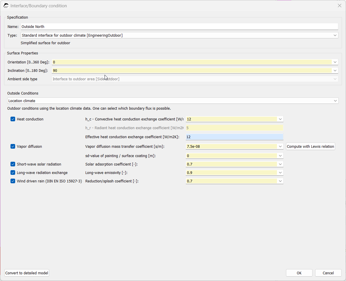
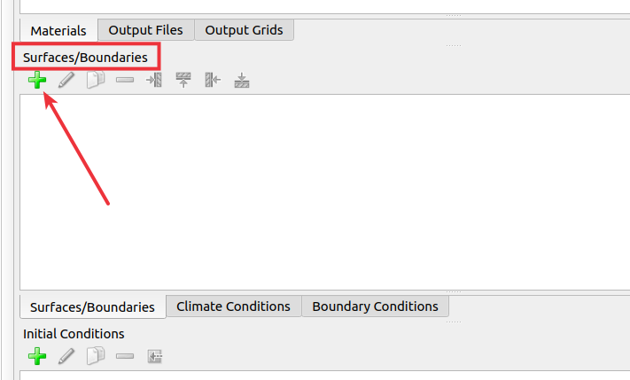
Another way to create the exterior boundary condition for the north wall is to use the button with the green plus sign. This creates a new exterior boundary condition.
The boundary conditions are now assigned to the corresponding locations. Select the interior plaster on the aerated concrete wall and click the “Inside” boundary condition. It is assigned to the right-hand side. Repeat this for the interior plaster on the brick wall, assigning the “Inside” boundary condition from above.
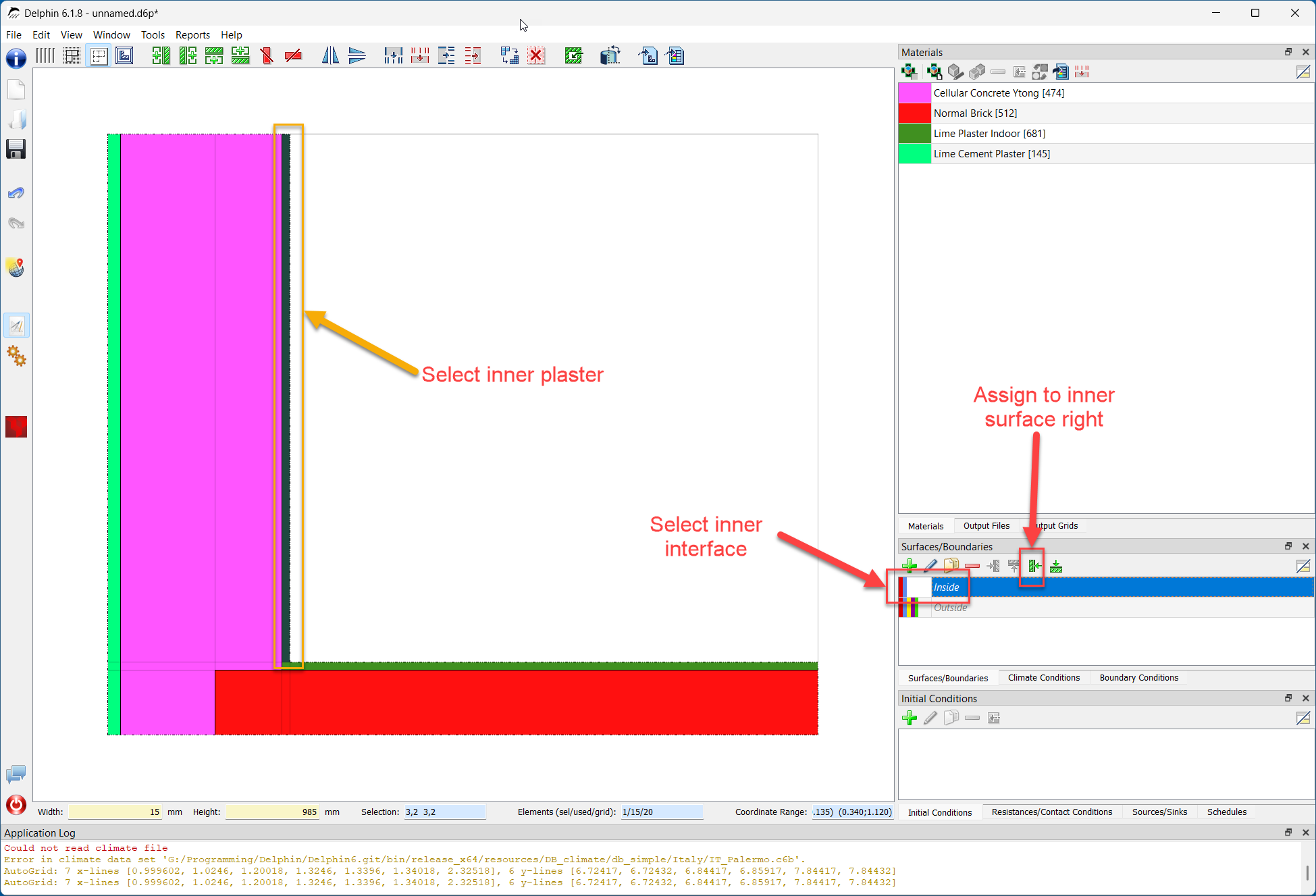
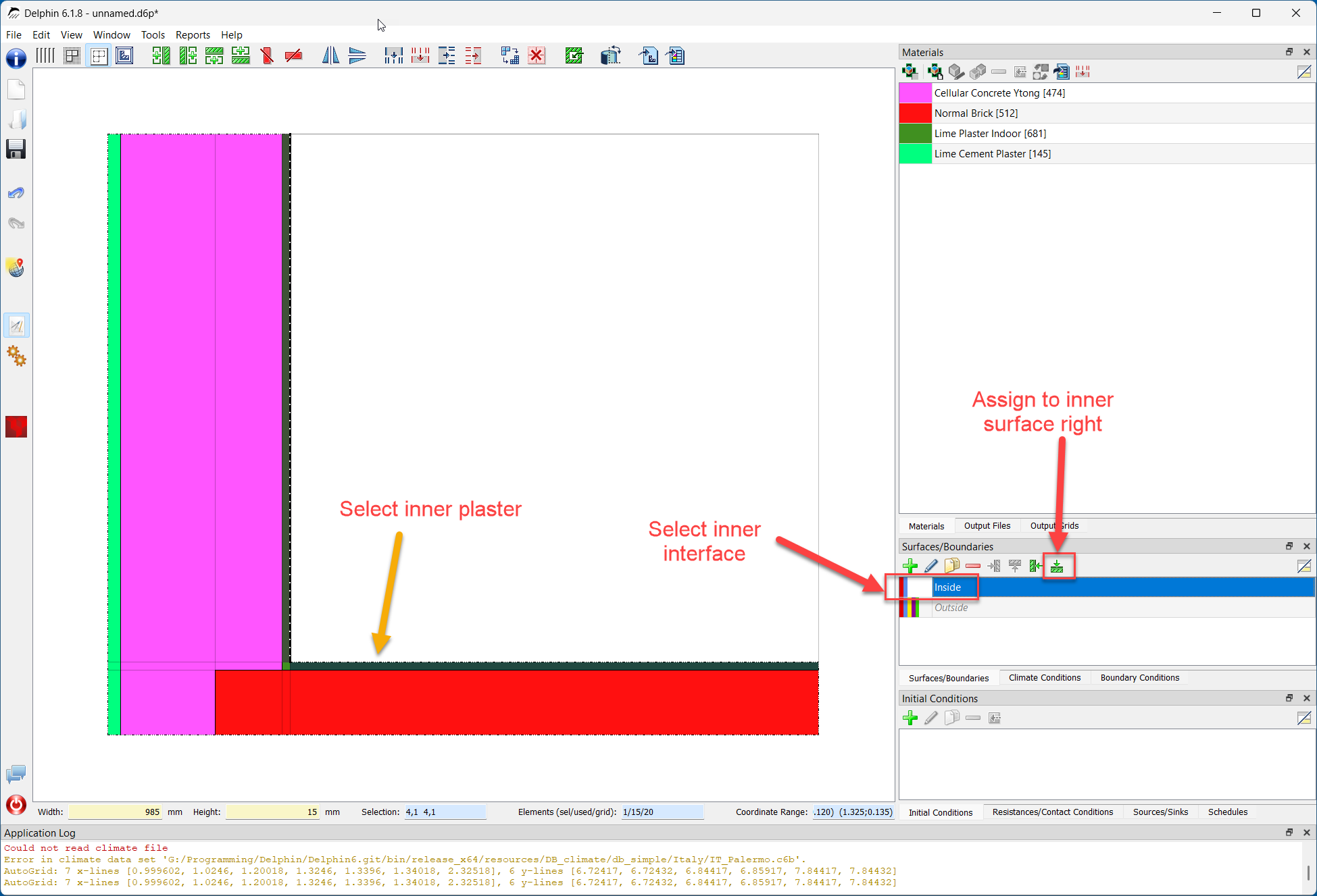
Finally, assign the exterior surface to the left side of the exterior plaster. Once all boundary conditions or surfaces have been assigned, the assignment can be checked by clicking a condition in the Surfaces/Boundaries window. For example, clicking “Indoor climate” highlights all interior room surfaces with a dashed line.
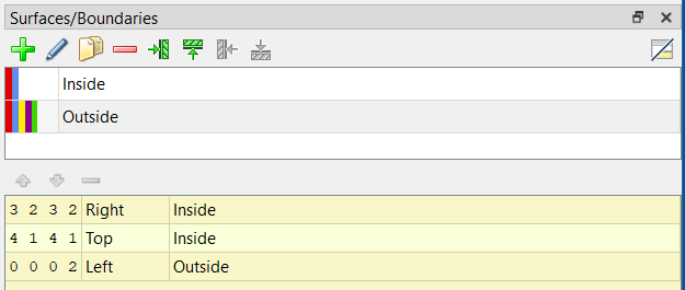
Each individual assignment can be checked in the assignment list of the Surfaces/Boundaries window (drag the lower edge upward). Three assignments should now be visible.
3. Generating the Discretization Grid
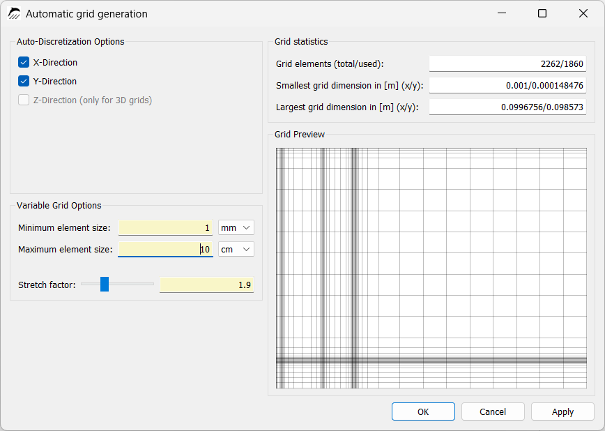
After creating the construction and assigning materials and boundary conditions, the discretization grid must be generated. The easiest way is to use the automatic discretization dialog. For this thermal bridge, both discretization directions x and y (the default for 2D constructions) must be selected. A value of 1 millimeter is appropriate for the minimum element thickness and should only be exceeded slightly. Here, a maximum element thickness of 100 mm and a scaling factor of 1.9 are selected.
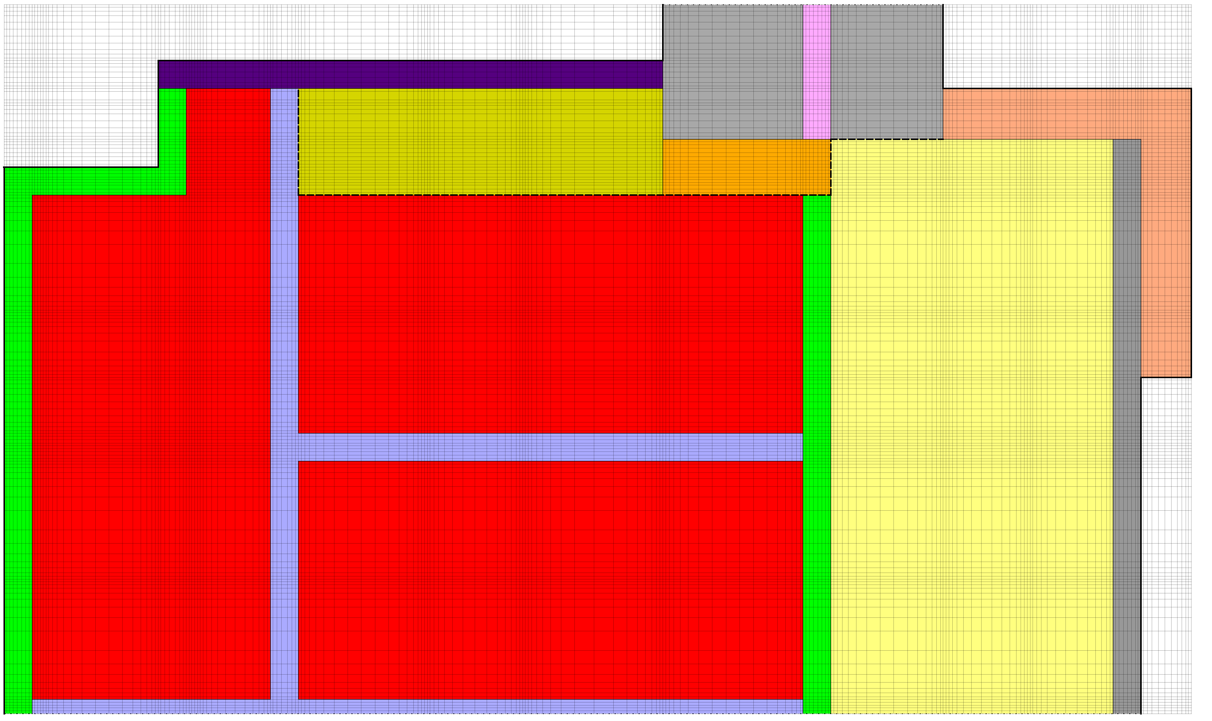
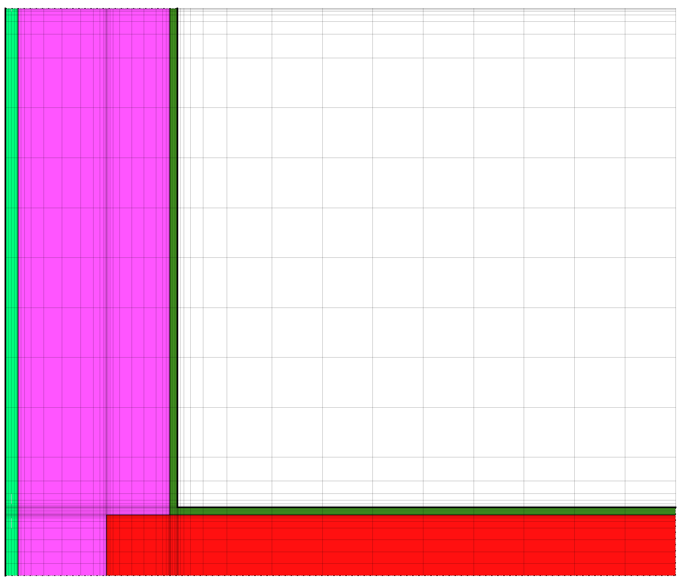
After discretization, the grid appears as follows:
The following notes explain the various functions of the status bar at the bottom of the construction grid.

The status bar displays various information when one or more elements are selected:
-
“Width/Height” displays the total width and height of all selected elements. The width and height of each individual cell can also be changed in this field. This function is disabled when multiple cells are selected.
-
“Selection” shows three numbers: the first is the number of currently selected elements, the second is the number of cells to which a material has been assigned, and the third is the total number of cells.
-
“Selection” and “Coordinate range” list the number and coordinates of the currently selected elements. The sequence starts with the first element in the horizontal direction, followed by the first selected element in the vertical direction, starting at the lower left. The last element in the horizontal direction and finally in the vertical direction follow (DELPHIN starts at “0”, not “1”).
Automatic discretization generates a grid that becomes finer toward the boundaries, i.e. toward construction surfaces (climate) and material interfaces. It is therefore easier to assign surface conditions before discretization.
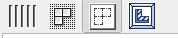
The buttons shown above, at the upper left of the construction window, change the display of the geometric model. From left to right, they allow you to switch between proportional and equidistant element display, show or hide construction lines, show or hide discretized-element lines, and fit the complete construction optimally into the window.
4. Outputs
For a simple thermal bridge, the temperature field is primarily used for a rough visual analysis, for example to identify the region with the lowest temperatures. For the structural design of a detail and verification in accordance with applicable guidelines, however, temperatures and relative humidity values in critical regions, especially on interior wall surfaces, are important. Heat fluxes across the interior surface may also be useful for quantifying heat losses in thermal-bridge regions. The post-processor allows temperatures and other quantities at specific points, as well as profiles along section lines, to be visualized and evaluated over time. In this example, the temperature field is generated first. If corresponding data are available (time series of temperature and relative humidity), the probability of mold growth can also be calculated.
The project wizard contains several predefined outputs. In this case, these are:
-
Temperature, relative humidity, and water-content profiles or fields
-
Moisture mass integral
A variety of custom outputs can be defined in the “Output files” field. The following screenshot shows the definition of the mean temperature output [Mean] in an area or at a specific point. It is advisable to choose a name that clearly identifies exactly what is being stored.
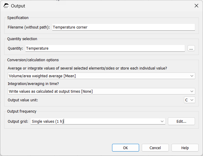
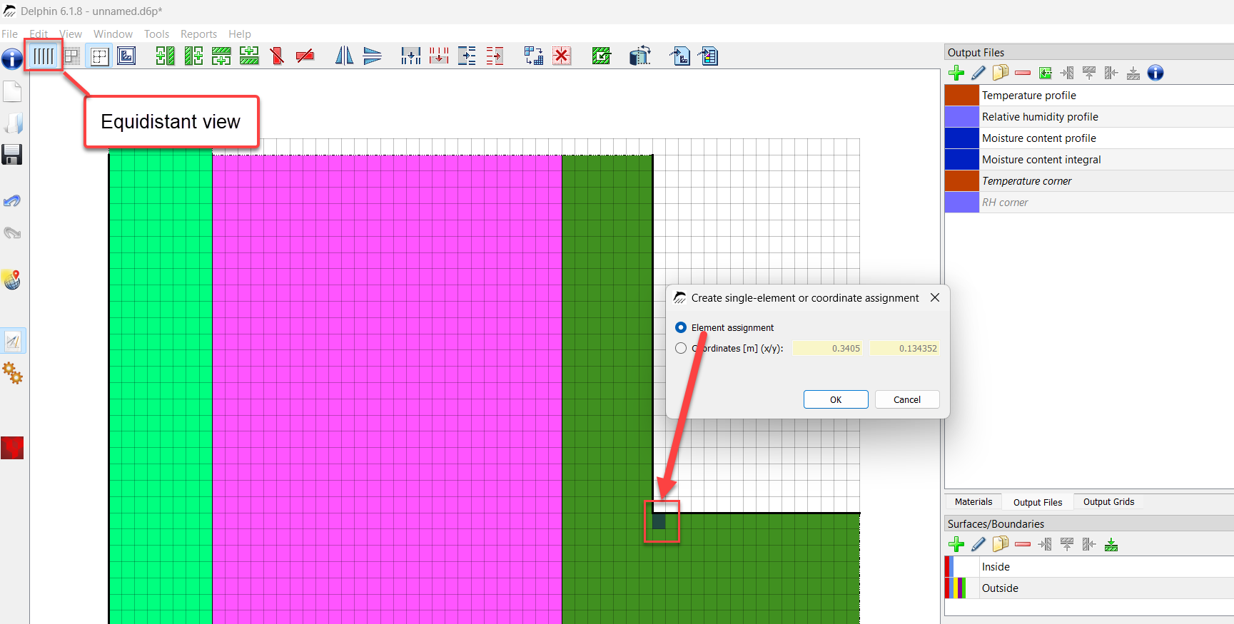
An output for relative humidity can be created in the same way. A faster method is to simply copy the temperature output that was just generated. Both outputs should be assigned to the critical point of the construction, the interior corner. Since the discretized elements are quite small, it is usually more convenient to use the equidistant display when assigning outputs to individual elements.
The relative humidity at the corner can also be determined in order to assess a potential mold risk. The following settings are used for the output and assignment:
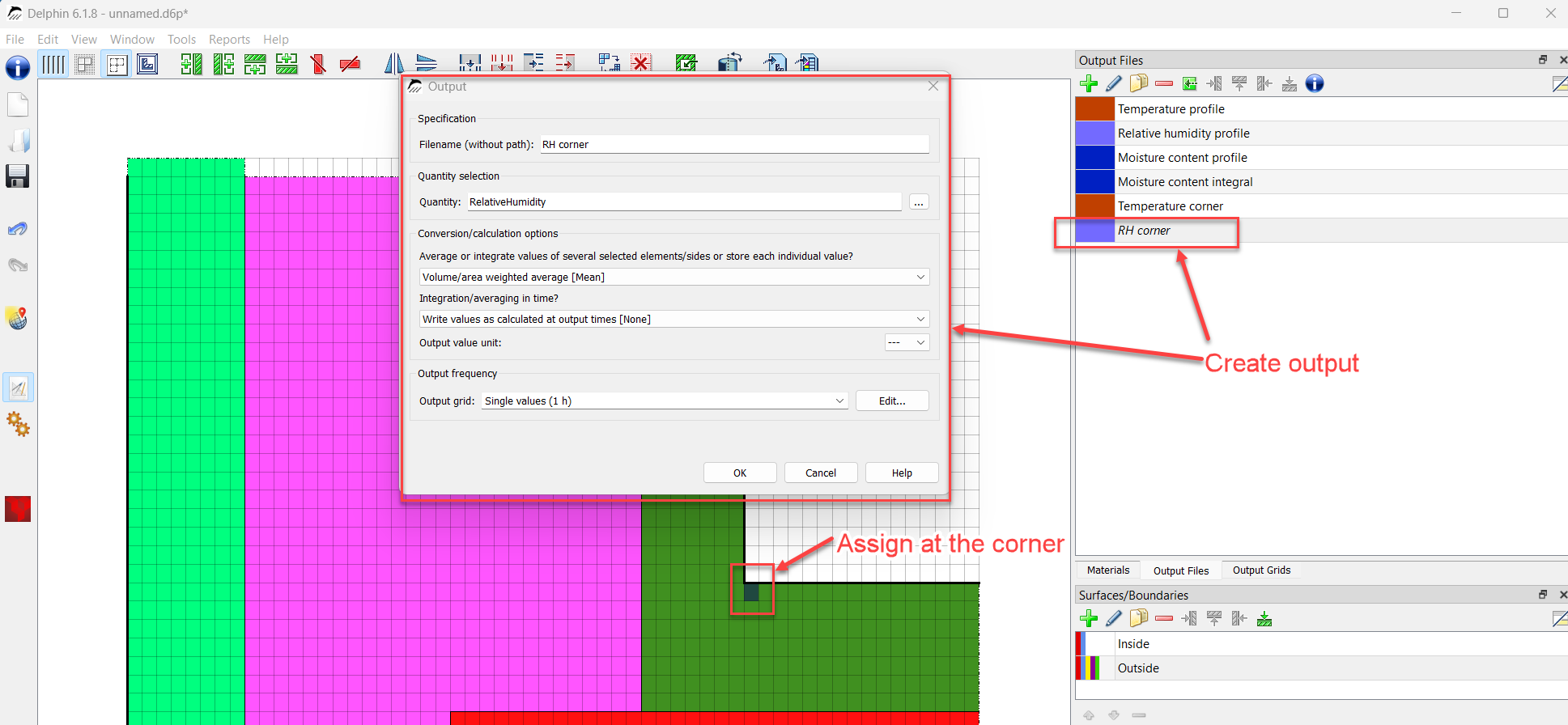
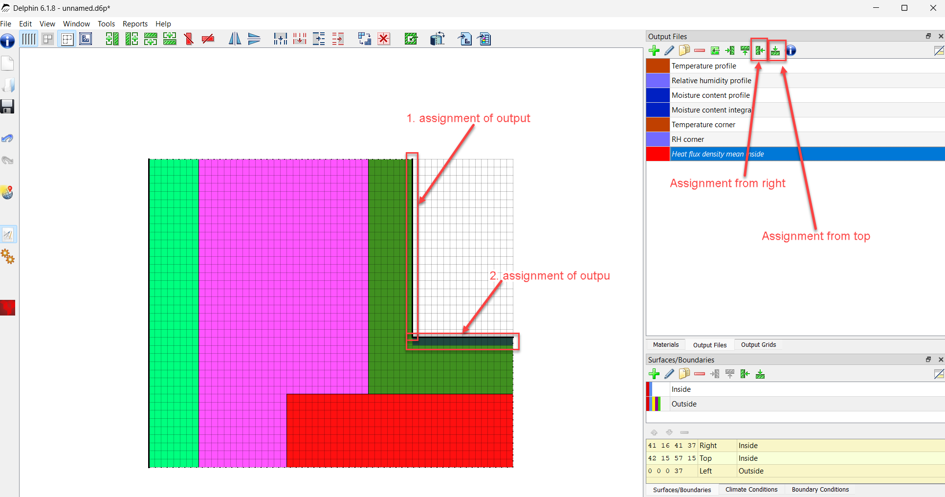
DELPHIN allows outputs to be assigned to one or more elements or to coordinates. Here, the outputs are assigned to a single element. The next output is defined for heat flux. In this case, two outputs are required.
For flux outputs, two different definitions must be observed:
-
Fluxes at construction boundaries are positive for incoming and negative for outgoing quantities
-
Fluxes within the field (i.e. inside the construction) depend on the direction (see below)
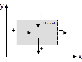
If a selection contains both field elements and elements at boundaries, the definitions for field conditions are used. A flux output can also be assigned to different element sides. In this case, the assignment is performed successively for both sides. For an area-/volume-averaged output definition, the area-/volume-averaged value for both sides is then output, for example at boundaries. In such a case, first create the output and then assign it successively to the different boundaries.
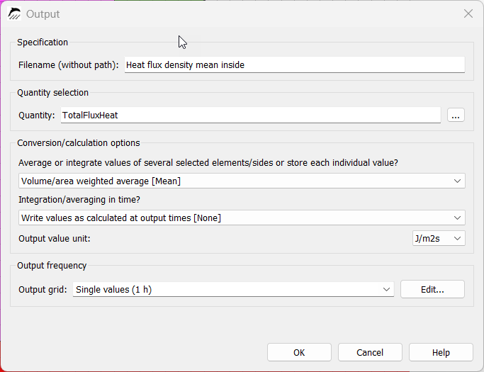
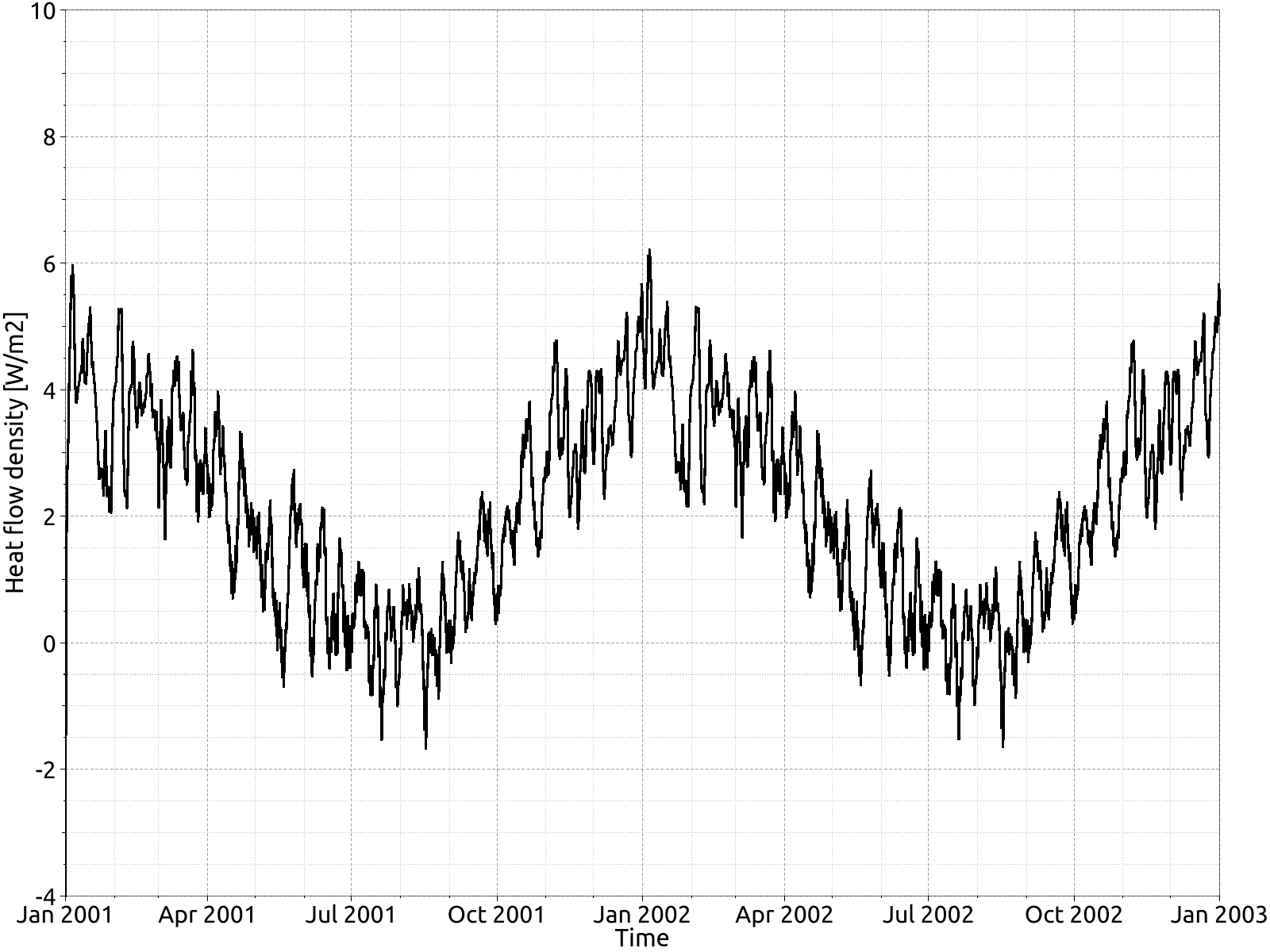
The following output has been generated for the heat flux across the interior surface:
5. Evaluation - Post-processing
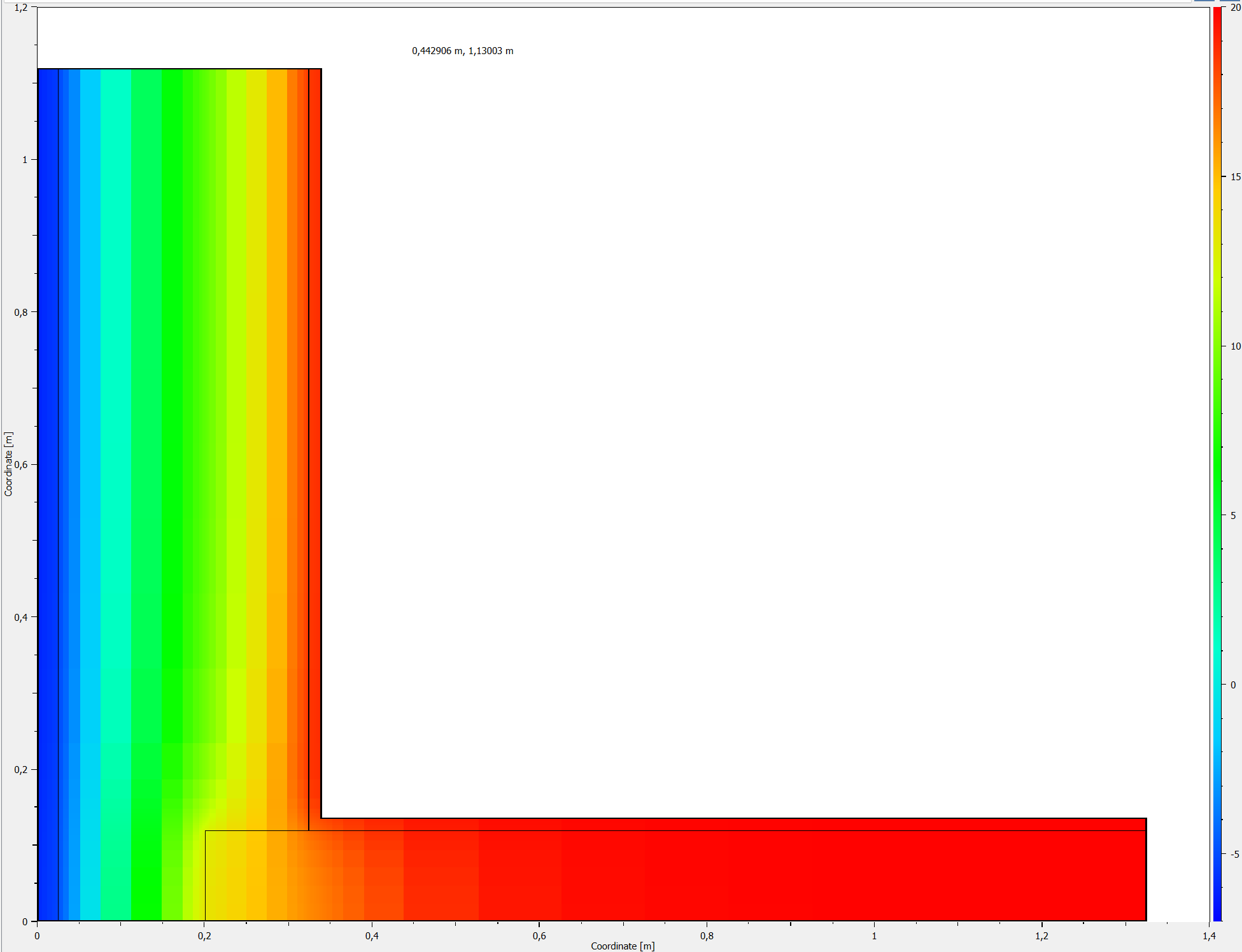
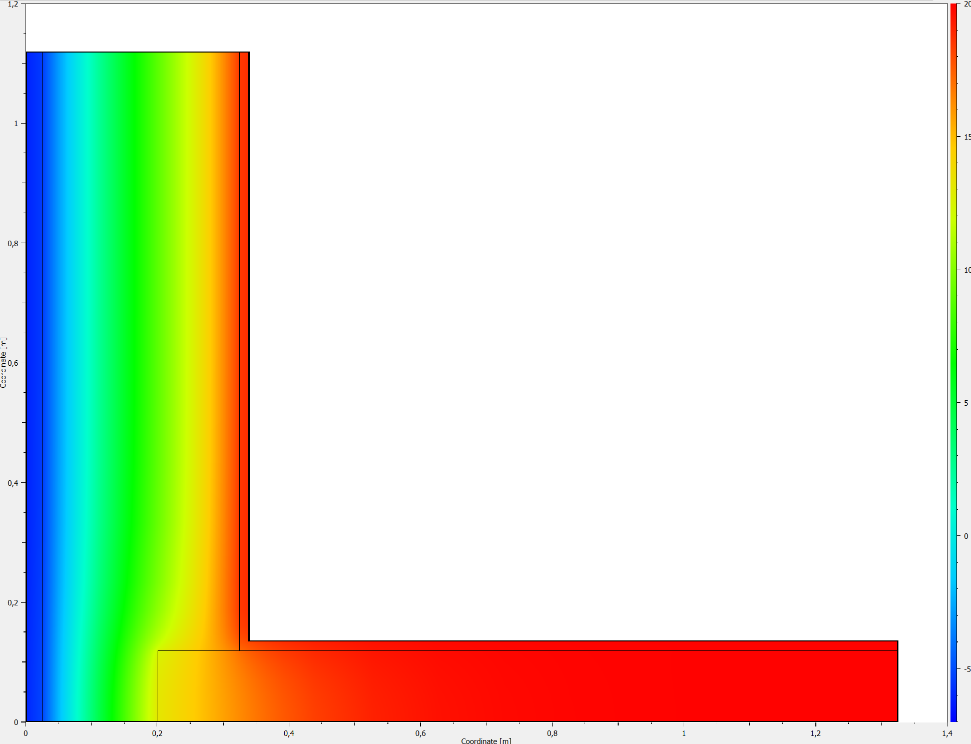
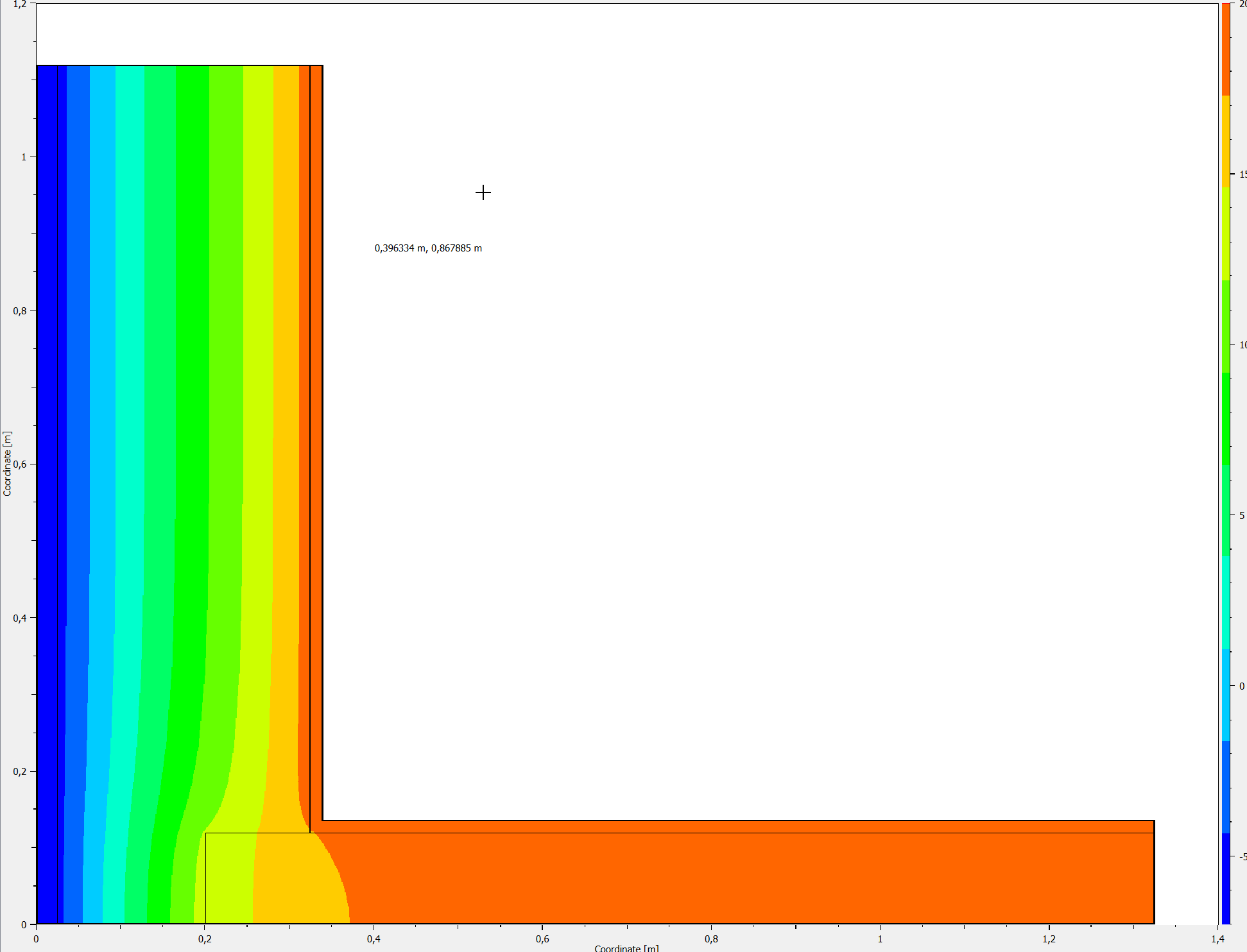
More information about the post-processor is provided in Tutorial 3. The following gives a brief overview of the PostProc 2 post-processor (>> File >> Settings >> External Programs). The next figure shows the temperature field on January 15 in interpolated (left) and non-interpolated mode (right). In non-interpolated mode, the discretized elements are clearly visible.
The temperature field with isotherms for the same point in time is shown in the next figure.
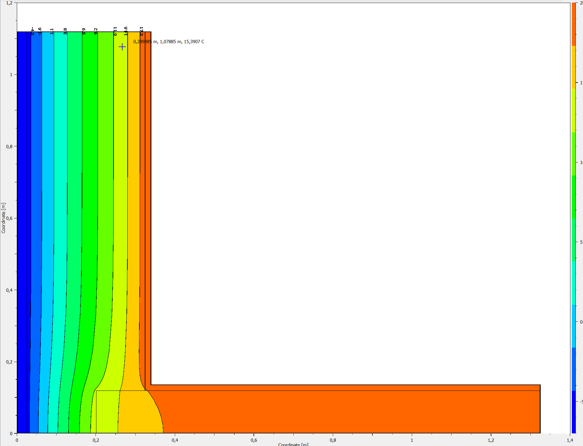
These types of diagrams can be used, for example, to assess whether the selected wall lengths reach the undisturbed region. This is achieved quickly for the interior wall, whereas the selected length for the exterior wall is only just sufficient.
The DELPHIN post-processor also allows two y-axes with different units to be used. The next (edited) figure shows temperature and relative humidity at the critical point, the interior corner.
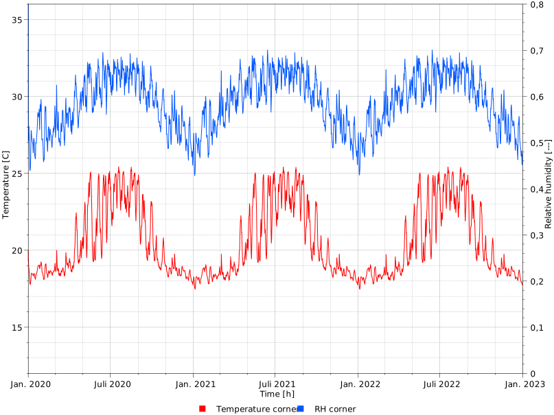
Since critical indoor relative-humidity values (approximately > 75% RH) are reached at times in this construction, the mold risk is assessed here.
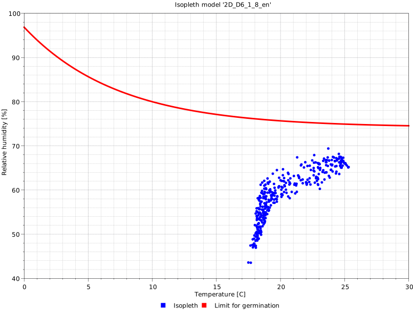
The diagram shows that high indoor temperatures in summer combined with high relative humidity (>75%) result in a mold risk on approximately 4 days over a total simulation period of 3 years = 26,280 days. This value is very small relative to the total simulation period and can be regarded as rather uncritical because the maximum duration of an individual period is < 24 h.
The following diagram shows the heat flux across the interior surfaces.
6. Automatic Report
6.1. Settings for Standard Assessments
First, various settings can be configured for the report. In the following dialog, the moisture accumulation of the entire construction and the risk of frost damage can be assessed in the automatically generated report. Assessment of moisture accumulation in each individual layer and the risk of mold growth cannot be enabled in the report for a 2D construction.

6.2. Input Data
A new feature in DELPHIN version 6.1.8 is the automatic report for 2D constructions. Various automatically generated reports can be opened from the “Report” menu in the upper menu bar. First, we will look at the input data.

The window shows three different subfolders on the right-hand side, each containing different settings.
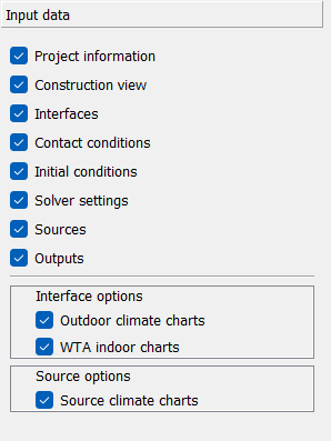
Various inputs can be displayed in the report; conditions that do not exist are initially not selected automatically.
First, the construction is shown with the assigned materials and color-coded boundary conditions. The following figures provide separate representations of these boundary conditions with detailed information on the selected properties.
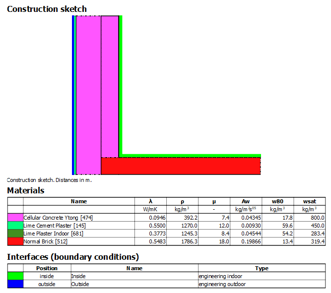
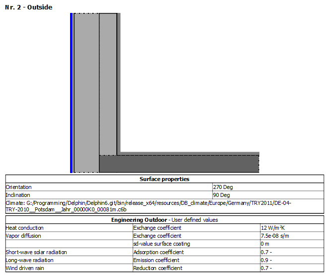
There is also a subfolder for drawing settings, where, for example, the size of the figures and the assignment of selected outputs can be specified.
6.3. Assessment Report
An automatically generated report is also available for assessing moisture accumulation and the risk of frost damage. Assessment of mold risk is not possible because the orientation of the interior boundary condition is user-defined rather than determined automatically.

The report contains various sections that can be enabled or disabled individually. The following figure highlights the three subfolders on the right-hand side of the window. The “General View” folder allows page numbers in the footer to be shown or hidden and the font and font size to be adjusted.
In the “Output files” folder below, various outputs can be included in the report.
| General report settings | Report outputs |
|---|---|
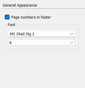
Figure 67. General report settings
|
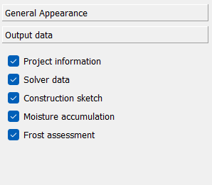
Figure 68. Report outputs
|
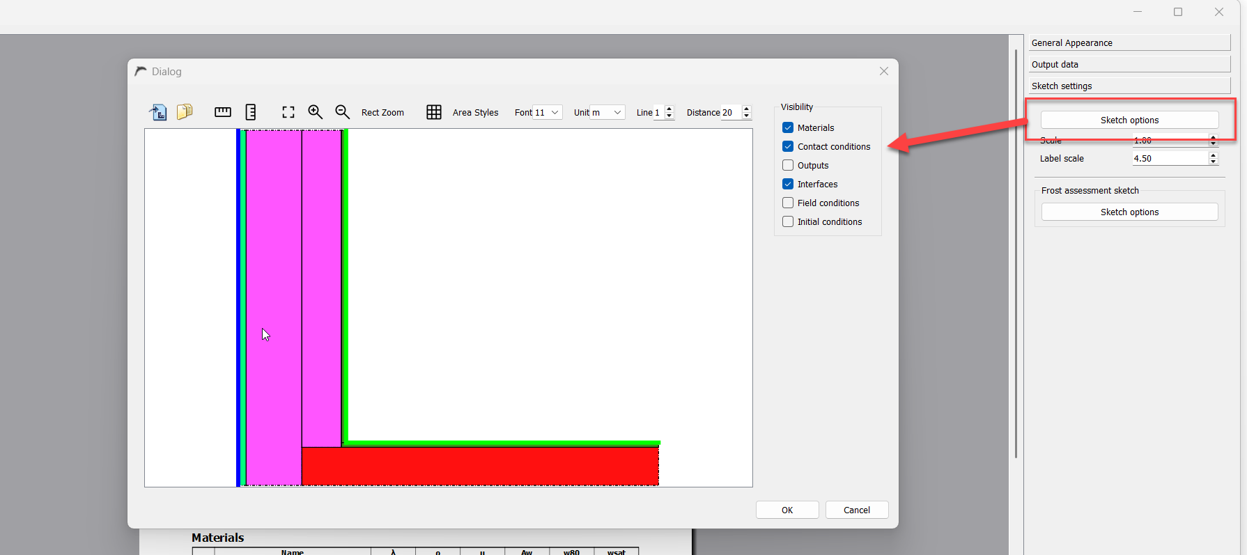
Enabling the project information, solver data, and construction drawing provides transparent documentation of the underlying boundary conditions and geometric modeling. The project information can be configured in the menu under Report > Project Information.
For this example, the moisture-accumulation assessment should be enabled.
A new section then appears in the report, showing moisture accumulation in the entire construction as a diagram and providing a brief assessment.
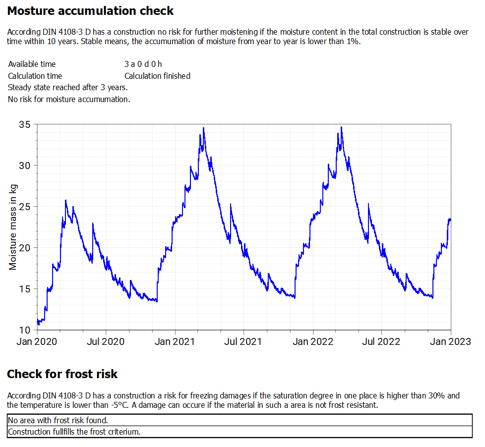
In this example, according to the report comment, there is no risk of moisture accumulation. The diagram shows that the construction dries continuously and reaches its equilibrium moisture content during the summer months. Therefore, there is no risk of moisture accumulation, as also stated in the report.
A frost assessment can also be performed. To do so, select the corresponding item in the “Output data” folder using the blue check box. In the following example, there is no risk of frost damage. A frost risk exists if frost-sensitive materials have a water saturation level of more than 30% at temperatures of -5 °C or below. According to DIN 4108-3, Annex D, the critical 10 mm of the affected material layer must be examined.